U.S. Department of Transportation
Federal Highway Administration
1200 New Jersey Avenue, SE
Washington, DC 20590
202-366-4000
Federal Highway Administration Research and Technology
Coordinating, Developing, and Delivering Highway Transportation Innovations
 |
| This report is an archived publication and may contain dated technical, contact, and link information |
|
Publication Number: FHWA-RD-01-165 Date: March 2002 |
Previous | Table of Contents | Next
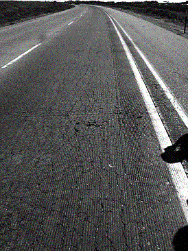
The South Dakota Department of Transportation (SDDOT) provided this project as a pavement with a history of durability problems. In particular, the pavement is experiencing surface or map cracking over the entire pavement surface. This project represents the primary case study site in the dry-freeze climatic region. The area receives approximately 400 mm of precipitation each year and has a freezing index of 684 °C-days.
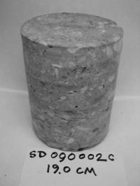
This 14-km-long project is located on I-90 near Spearfish, South Dakota and extends from milepost 19.8 to milepost 28.5 in both directions. Table 3-2 provides a summary of the specific design features for this project.
Table 3-2. Summary of design features for SD-090-019.
|
Category |
Design Feature |
Description |
|---|---|---|
|
General |
Project limits |
MP 19.8 - 28.5 |
|
Highway type |
Divided |
|
|
Number of lanes |
4 |
|
|
Direction |
Eastbound/westbound |
|
|
Construction date |
1968 |
|
|
Cumulative ESALs |
~2,250,000 |
|
|
Pavement |
Pavement type |
JRCP |
|
PCC slab thickness |
200 mm |
|
|
Base |
75-mm lime-treated gravel |
|
|
Subbase |
150-mm lime-treated subgrade |
|
|
Subgrade type |
Red clay |
|
|
Transverse |
Joint spacing |
12.3 m |
|
Joint skew |
None |
|
|
Load transfer |
25-mm dowels |
|
|
Sealant type |
Silicone |
|
|
Longitudinal |
Load transfer |
|
|
Sealant type |
Hot-pour |
|
|
Outer |
Surface type |
AC |
|
Width |
3.0 m |
|
|
Inner |
Surface type |
AC |
|
Width |
1.2 m |
|
|
Climatic |
Region |
Dry-freeze |
|
Annual precipitation* |
400 mm |
|
|
Freezing index* |
684 °C-days |
The project is a four-lane divided highway, and the same design was placed in both the eastbound and westbound lanes. It is a jointed reinforced concrete pavement (JRCP) containing wire mesh reinforcement. The joints are spaced at 12.3-m intervals and contain 25-mm dowel bars. The longitudinal centerline joint is sealed with a hot-pour asphalt sealant, whereas the transverse joints are sealed with a silicone sealant. The pavement structure consists of a 200-mm JRCP, a 75-mm lime-treated gravel base, and a 150-mm lime-treated subgrade. The subgrade is a red clayey soil. There are no provisions for subsurface drainage. The inside and outside shoulders are AC-surfaced and are 1.2 and 3.0 m wide, respectively.
After an initial investigation, the survey team selected two sections-one each in the inside and outside traffic lanes-to be surveyed in order to evaluate the differences between lanes. Section 001 is located in the eastbound, inside traffic lane beginning at milepost 23.1. This section was constructed in a cut section of approximately 10 m. Section 002 is also located in the eastbound direction but in the outside traffic lane and begins at milepost 24.5. This section was constructed on approximately 3 m of fill material.
A summary of the distress survey results is provided in tables 3-3 and 3-4 for Sections 001 and 002, respectively. Overall, Section 001 appears to be in better structural condition than Section 002, as would be expected due to the lower traffic volumes on the inside traffic lane. Section 001 contains some low-severity transverse cracks, which are expected to occur on JRCP. Spalling occurs at 6 of the 14 transverse joints but only 1 has progressed to medium severity. The spalling appears to be due to the progression of MRD. Three small rigid patches, each of which is located along a transverse joint, are also present. Faulting is virtually nonexistent, averaging 0.6 and 0.7 mm measured at distances of 0.30 and 0.75 m from the slab edge.
Section 002 exhibits more distress and greater deterioration. Although low-severity transverse cracks are expected on JRCP, there are considerably more cracks as compared to Section 001. In addition, Section 002 also exhibits two medium-severity cracks and two high-severity cracks. Faulting is also much more significant, averaging 3.7 and 4.2 mm at 0.30 and 0.75 m from the slab edge. Another distress that is more significant on Section 002 is patching. A high-severity flexible patch is observed, as are 10 low-severity and 2 moderate-severity rigid patches. Some of the rigid patches are full-depth patches at transverse joints, indicating that the joints were likely badly deteriorated at one time. Five of the 14 transverse joints exhibit spalling, including 2 that have progressed to moderate severity.
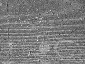
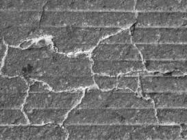
During the field surveys, the attributes of the MRD were characterized. Although a definitive diagnosis cannot be made in the field, it is important to evaluate the attributes of the MRD as well as the effect these distresses have on pavement performance. A summary of the MRD characterization for both sections is provided in table 3-5. Figures 3-2 through 3-4 show some the typical conditions observed on the two test sections.
Table 3-3. Summary of pavement condition surveys for SD-090-019-001.
|
Distress Type |
Distress |
Severity Level |
Comments |
|||
|---|---|---|---|---|---|---|
|
Low |
Moderate |
High |
||||
|
Cracking |
Corner Breaks |
number |
1 |
0 |
0 |
|
|
Longitudinal Cracking |
linear meters |
0.0 |
0.0 |
0.0 |
||
|
Transverse Cracking |
number of cracks |
12 |
0 |
0 |
||
|
linear meters |
14.7 |
0.0 |
0.0 |
|||
|
percent of slabs |
0 |
|||||
|
Transverse |
Sealant |
good condition |
silicone sealant |
|||
|
Spalling |
number |
5 |
1 |
0 |
||
|
linear meters |
1.4 |
0.4 |
0 |
|||
|
Faulting |
millimeters |
0.6 |
measured at 0.30 m |
|||
|
millimeters |
0.7 |
measured at 0.75 m |
||||
|
Width |
millimeters |
23.6 |
||||
|
Long. Joints |
Sealant |
fair condition |
hot-pour sealant |
|||
|
Spalling |
linear meters |
0.0 |
0.0 |
0.0 |
||
|
Shoulder Dropoff |
millimeters |
17.8 |
||||
|
Surface |
Map Cracking |
number of slabs |
13 |
all slabs affected |
||
|
square meters |
588.3 |
entire area |
||||
|
Scaling |
number of slabs |
0 |
||||
|
square meters |
0.0 |
|||||
|
Polished Aggregate |
square meters |
0.0 |
||||
|
Popouts |
number/sq. meter |
0.0 |
||||
|
Other |
Blowups |
number |
0 |
|||
|
Flexible Patches |
number |
0 |
0 |
0 |
||
|
square meters |
0.0 |
0.0 |
0.0 |
|||
|
Rigid Patches |
number |
3 |
0 |
0 |
||
|
square meters |
0.4 |
0.0 |
0.0 |
|||
|
Pumping/Bleeding |
number |
0 |
||||
|
linear meters |
0.0 |
|||||
Table 3-4. Summary of pavement condition surveys for SD-090-019-002.
|
Distress Type |
Distress Measure |
Severity Level |
Comments |
|||
|---|---|---|---|---|---|---|
|
Low |
Moderate |
High |
||||
|
Cracking |
Corner Breaks |
number |
1 |
0 |
0 |
|
|
Longitudinal Cracking |
linear meters |
0.0 |
0.0 |
0.0 |
||
|
Transverse Cracking |
number of cracks |
44 |
2 |
2 |
||
|
linear meters |
60.9 |
7.4 |
7.4 |
|||
|
percent of slabs |
31 |
|||||
|
Transverse |
Sealant |
good condition |
silicone sealant |
|||
|
Spalling |
number |
3 |
2 |
0 |
||
|
linear meters |
1.1 |
1.9 |
0.0 |
|||
|
Faulting |
millimeters |
3.7 |
measured at 0.30 m |
|||
|
millimeters |
4.2 |
measured at 0.75 m |
||||
|
Width |
millimeters |
17.2 |
||||
|
Long. Joints |
Sealant |
fair condition |
hot-pour sealant |
|||
|
Spalling |
linear meters |
0.0 |
0.0 |
0.0 |
||
|
Shoulder Dropoff |
millimeters |
23.6 |
||||
|
Surface |
Map Cracking |
number of slabs |
13 |
all slabs affected |
||
|
square meters |
579.0 |
entire area |
||||
|
Scaling |
number of slabs |
0 |
||||
|
square meters |
0.0 |
|||||
|
Polished Aggregate |
square meters |
0.0 |
||||
|
Popouts |
number/sq. meter |
0.0 |
||||
|
Other |
Blowups |
number |
0 |
|||
|
Flexible Patches |
number |
0 |
0 |
1 |
||
|
square meters |
0.0 |
0.0 |
0.5 |
|||
|
Rigid Patches |
number |
10 |
2 |
0 |
||
|
square meters |
15.4 |
3.8 |
0.0 |
|||
|
Pumping/Bleeding |
number |
0 |
||||
|
linear meters |
0.0 |
|||||
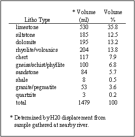
Table 3-5. Summary of MRD characterization for SD-090-019.
|
Description |
Section 001 |
Section 002 |
Comments |
|
|
Cracking |
Location |
Entire slab |
Entire slab |
More significant at slab corners |
|---|---|---|---|---|
|
Orientation/shape |
Criss cross |
Corners: semi-circle Center: transverse |
||
|
Extent |
Entire slab |
Entire slab |
||
|
Crack size |
Hairline |
Hairline |
||
|
Staining |
Location |
Joints/cracks |
Joints/cracks |
|
|
Color |
Brownish gray |
Dark gray |
||
|
Exudate |
Present |
None |
Yes |
Corners only |
|
Color |
n/a |
Dark gray/white |
||
|
Extent |
n/a |
Low |
||
|
Scaling |
Location |
None |
None |
|
|
Area of surface |
n/a |
n/a |
||
|
Depth |
n/a |
n/a |
||
|
Vibrator |
Visible |
None |
None |
|
|
Discolored |
n/a |
n/a |
||
|
Distressed |
n/a |
n/a |
||
|
Change in texture |
n/a |
n/a |
||
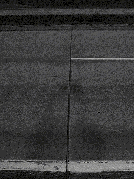
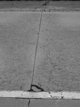
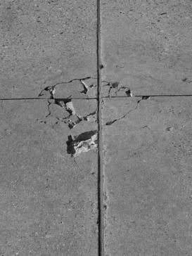
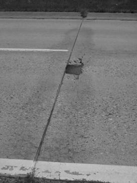
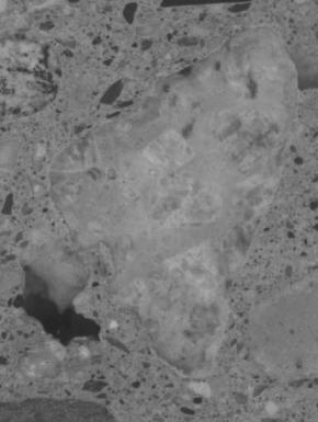
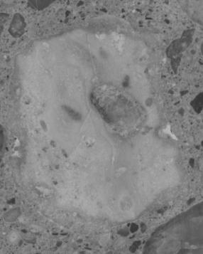
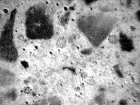
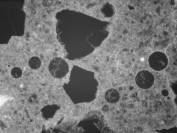
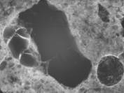
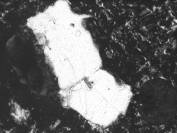
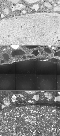
Figure 3-2. Typical distress manifestation observed on SD-090-019-002.
Figure 3-3. Typical distress manifestation observed on SD-090-019, Sections 1 and 2.
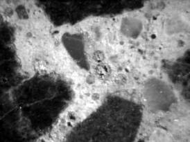
Figure 3-4. Typical distress manifestation observed on SD-090-019-002.
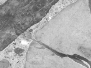
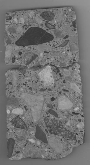
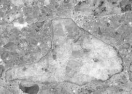
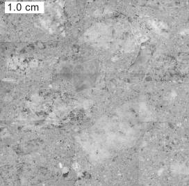
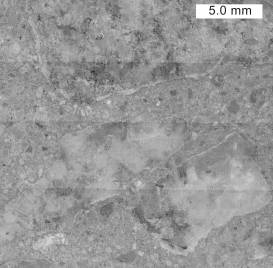
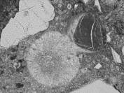
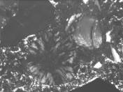
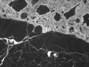
On both pavement sections, map cracking was observed throughout the entire area. On Section 001, the cracks appear to be confined to the upper 50 mm at the pavement surface. The majority of cracks run perpendicular to the centerline, but there are some cracks that run parallel to the centerline. The combination of cracks forms a criss-cross pattern on the surface. Although the cracking pattern is similar on Section 002, the transverse cracks on Section 001 are more pronounced and some are opened at the surface.
On Section 001, the area around the joints is discolored, showing a brownish-gray staining. However, the cracking pattern around the joints is similar to the slab interior. The MRD has progressed at a few of the slab corners and spalling has occurred. There is no exudate from the cracks on this section.
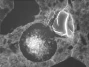
Section 002 exhibits a different cracking pattern along the joints. The cracking and staining form a semi-circular pattern, widening at the slab corners. A dark gray staining is observed around both the longitudinal and transverse joints. Unlike Section 001, exudate is observed at some cracks, particularly cracks located near a joint. The exudate is either a dark gray or white substance.
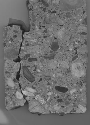
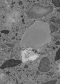
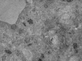
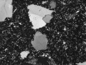
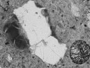
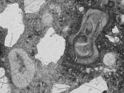
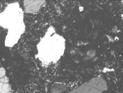
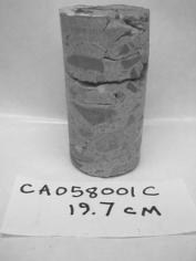
Core Selection/Visual Inspection
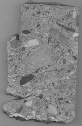
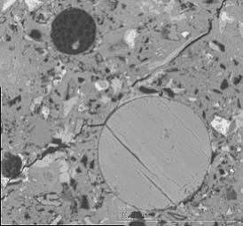
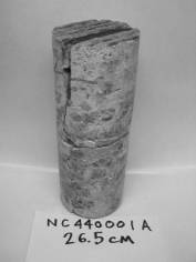
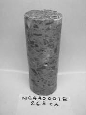
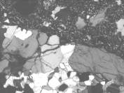
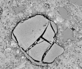
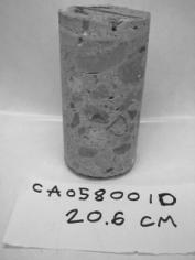
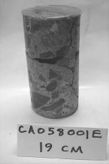
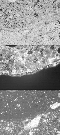
Based upon the field survey, distress was detected at joints and near slab corners. Photos of typical distresses are shown in figure 3-5. To look at concrete from more than one slab, Cores B and D were selected from Section 001 and Cores A, B, and C were selected from Section 002. All cores were cut to produce slabs for examination with stains.
|
|
|
|
||
|
(a) Section 001, Core B |
(b) Section 002, Core A |
(c) Section 002, Core C |
Figure 3-5. Core specimens from SD-090-019.
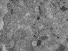
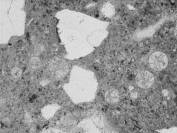
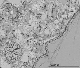
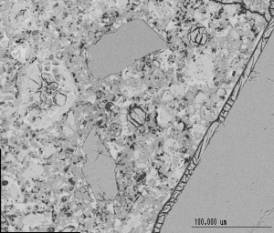
Mix proportions were estimated by inspecting the cores visually before and after slicing. In this case, detailed construction records were unavailable to verify the mix design. The concrete was well consolidated with no apparent segregation or parallelism of the aggregates. No scaling or sub-parallel cracking was apparent on these sites. The embedded steel was at a sufficient depth to prevent corrosion and no entrapped water voids were seen under aggregates or embedded steel. Surface cracking was apparent that was not related to plastic shrinkage cracking.
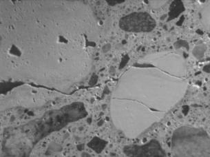
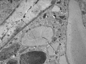
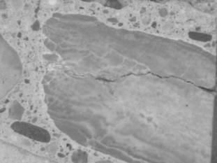
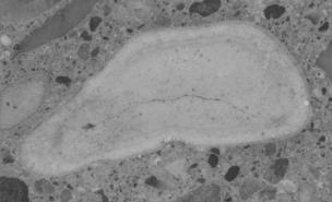
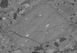
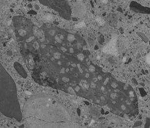
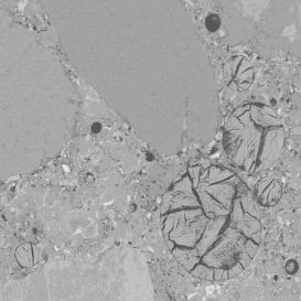
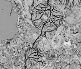
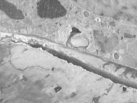
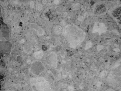
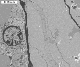
The stereo optical microscope was used to first examine polished slabs cut from each core to assess the general condition of the concrete. Typical micrographs of interesting features are presented in figures 3-6 and 3-7. The aggregate type was determined to be a natural gravel with a varied lithology including limestone, siltstone, dolomite, and rhyolite as the main rock types for the coarse aggregate. Many of the rhyolite particles had small feldspar inclusions. The fine aggregates contained the same rock types seen in the coarse aggregate in addition to shale, sandstone quartzite, and granite. Cracks passing through the paste also passed through aggregates. Reaction rims were visible along with secondary infilling in cracks and air voids. A yellow to white "soft" crumbly siltstone constituent of the coarse aggregate natural gravel is frequently cracked, with the cracks extending into the surrounding cement paste, and occasional white deposits in cracks. Aggregate particles that were volcanics or rhyolites appear to be reactive.
Figure 3-6. Stereo optical micrographs of typical cracking pattern associated with porous siltstone aggregate SD-090-019.
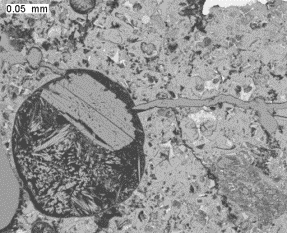
Figure 3-7. Stereo optical micrograph showing gel deposits in SD-090-019 aggregates.
The stereo microscope was also used to perform a modified point count in accordance with ASTM C 457. As part of the modified point count, the volume fractions of paste and aggregate were also determined to confirm mix volumetrics. The results of this analysis are given in table 3-6.
Table 3-6. Results of ASTM C 457 for concrete from SD-090-019.
|
Original |
Existing |
Volume Percent |
|||||
|---|---|---|---|---|---|---|---|
|
Core |
Air Content |
Spacing Factor |
Air Content |
Spacing Factor |
Paste |
Coarse Aggregate |
Fine Aggregate |
|
Site 1 Core A |
6.0 |
0.1274 |
6.0 |
0.1375 |
25.6 |
47.9 |
20.5 |
|
Site 1 Core D |
5.7 |
0.1073 |
5.7 |
0.1047 |
26.4 |
52.0 |
15.9 |
|
Site 2 Core C |
5.5 |
0.1089 |
5.4 |
0.1114 |
27.16 |
41.5 |
25.8 |
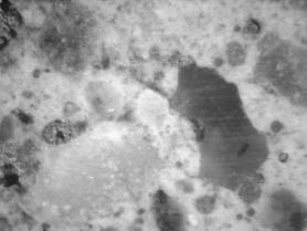
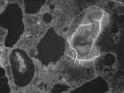
The sodium cobaltinitrite/rhodamine B staining tests were applied and a number of aggregates were identified as being susceptible to alkali-silica reactivity (ASR). The phenolphthalein staining method was used to determine the depth of carbonation on freshly cut surfaces. Slabs cut from the analyzed cores were tested for depth of carbonation with no core having a depth of carbonation greater than 2 mm below the road surface. Barium chloride/potassium permanganate stain was used to identify sulfate minerals. Examples of the stained slabs are presented in figures 3-8 through 3-11.
|
|
(b) Stereo optical micrograph of reactive porous siltstone particle |
|
|
(a) Stained slab |
(c) Stereo optical micrograph of reactive volcanic particle |
Figure 3-8. Slab 1B stained with sodium cobaltinitrite/rhodamine B from SD-090-019-001.
|
|
(b) Stereo optical micrograph of reactive rhyolite particle |
|
|
|
||
|
(a) Stained slab |
(c) |
Figure 3-9. Slab 1B stained with sodium cobaltinitrite/rhodamine B from SD-090-019-001.
|
|
|
|
|
(a) Stained slab |
(b) Reactive aggregate particle |
|
|
|
|
|
|
(c) ASR gel filled void |
(d) Reactive aggregate particle |
Figure 3-10. Slab 2B stained with sodium cobaltinitrite/rhodamine B from SD-090-019-002.
|
|
|
|
|
(a) Ettringite filled voids on polished surface |
(b) Ettringite filled voids on polished surface |
|
|
|
|
|
|
(c) Ettringite filled voids on unpolished surface |
(d) Ettringite filled voids on unpolished surface |
Figure 3-11. Stereo optical micrographs of air voids filled with sulfate minerals stained with potassium permanganate (note differences due to polishing).
Petrographic Optical Microscopy
Based upon stereo microscope observations and staining, thin sections were prepared from the selected cores. Surfaces were sectioned from the core adjacent to stained sections to avoid contamination from the stains. The reactive coarse aggregates were primarily the siltstones and rhyolites, although others were noted as reactive. The shale was commonly associated with ASR in fine aggregate. In addition to cracking associated with ASR, other cracking of non-reacted siltstone aggregates was noted. The siltstone aggregates had a very porous microstructure as seen in thin section. These aggregates may be susceptible to aggregate freeze-thaw deterioration, leading to some of the cracking seen in the concrete. In addition to possible ASR and aggregate freeze-thaw deterioration, evidence of alkali-carbonate reactivity (ACR) was noted where densified paste regions or "halos" with a large amount of calcite were seen surrounding dolomite coarse aggregates (Spry et al. 1996). Secondary deposits within cracks and voids were identified. In addition to specific phases identified (e.g., ASR gel, calcite), ettringite was common as a secondary deposit. In addition to these diagnostic features, hydrocalumite (Friedel's salt) secondary deposits were found. Given the high chloride concentration needed to precipitate hydrocalumite, this is taken as a diagnostic feature of deicer attack. Petrographic micrographs are presented in figures 3-12 and 3-13.
Scanning Electron Microscopy (SEM)
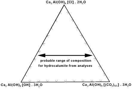
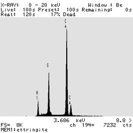
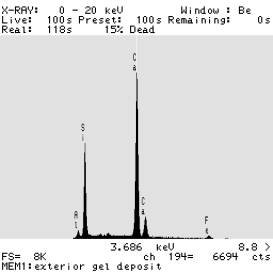
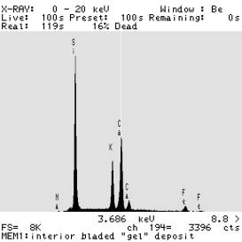
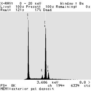
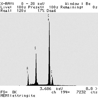
A conventional SEM was used to identify secondary deposits seen in the petrographic microscope examination to confirm those observations. Figure 3-14 containsa backscattered electron image showing an ettringite filled void, a crack filled with hydrocalumite, and characteristic x-ray spectra from each phase illustrating their compositions. The SEM analysis confirmed the petrographic analysis with regards to the composition of the secondary deposits. The phase identified as hydrocalumite was confirmed, as were the presence of ettringite and the composition of various ASR reaction products. The results of x-ray microanalyses of the ettringite and the hyrocalumite phases are presented in tables 3-7 and 3-8, respectively. Figure 3-15 presents the ternary diagram showing the probable range of composition for the hydrocalumite deposits.
 |
 |
|---|---|
 |
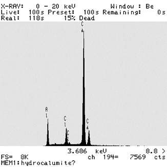 |
Figure 3-14. Ettringite (a) and hydrocalumite (b) infilling in void and crack, respectively. Example spectra from each phase are shown in (c) and (d), respectively.
|
Element |
Average |
Standard |
Dehydrated |
|---|---|---|---|
|
Na |
0.2 |
0.2 |
0.0 |
|
Mg |
0.0 |
0.0 |
0.0 |
|
Al |
7.9 |
0.3 |
6.9 |
|
Si |
0.3 |
0.1 |
0.0 |
|
S |
11.6 |
0.5 |
12.2 |
|
Cl |
0.2 |
0.1 |
0.0 |
|
K |
0.0 |
0.0 |
0.0 |
|
Ca |
31.2 |
0.6 |
30.6 |
|
Ti |
0.0 |
0.0 |
0.0 |
|
Mn |
0.0 |
0.1 |
0.0 |
|
Fe |
0.0 |
0.1 |
0.0 |
|
O |
- |
- |
48.8 |
|
H |
- |
- |
1.5 |
|
sum |
51.3 |
100.0 |
|
Element |
Average |
Standard |
Dehydrated |
Dehydrated OH- hydrocalumite |
Dehydrated |
|---|---|---|---|---|---|
|
Na |
0.0 |
0.1 |
0.0 |
0.0 |
0.0 |
|
Mg |
0.0 |
0.1 |
0.0 |
0.0 |
0.0 |
|
Al |
12.5 |
0.4 |
11.0 |
12.9 |
12.5 |
|
Si |
0.4 |
0.4 |
0.0 |
0.0 |
0.0 |
|
S |
0.0 |
0.0 |
0.0 |
0.0 |
0.0 |
|
Cl |
5.0 |
0.2 |
14.5 |
0.0 |
0.0 |
|
K |
0.0 |
0.1 |
0.0 |
0.0 |
0.0 |
|
Ca |
36.0 |
0.8 |
32.8 |
38.3 |
37.3 |
|
Ti |
0.0 |
0.0 |
0.0 |
0.0 |
0.0 |
|
Mn |
0.0 |
0.1 |
0.0 |
0.0 |
0.0 |
|
Fe |
0.3 |
0.2 |
0.0 |
0.0 |
0.0 |
|
C |
- |
- |
0.0 |
0.0 |
2.8 |
|
|
- |
- |
39.2 |
45.9 |
44.6 |
|
H |
- |
- |
2.5 |
2.9 |
2.8 |
|
sum |
54.2 |
100.0 |
100.0 |
100.0 |
Figure 3-15. Ternary diagram showing the probable range of composition for the hydrocalumite deposits analyzed from SD-090-019.
Ion chromatography was used to analyze the sulfate content of soil samples taken from the grade below the individual core holes. The complete analysis is presented in the final report. To summarize, the soil base below the test sites would be classified as a negligible sulfate exposure using the criteria set forth in ACI 201.2R-92 Guides to Durable Concrete.
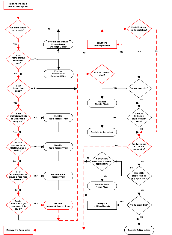
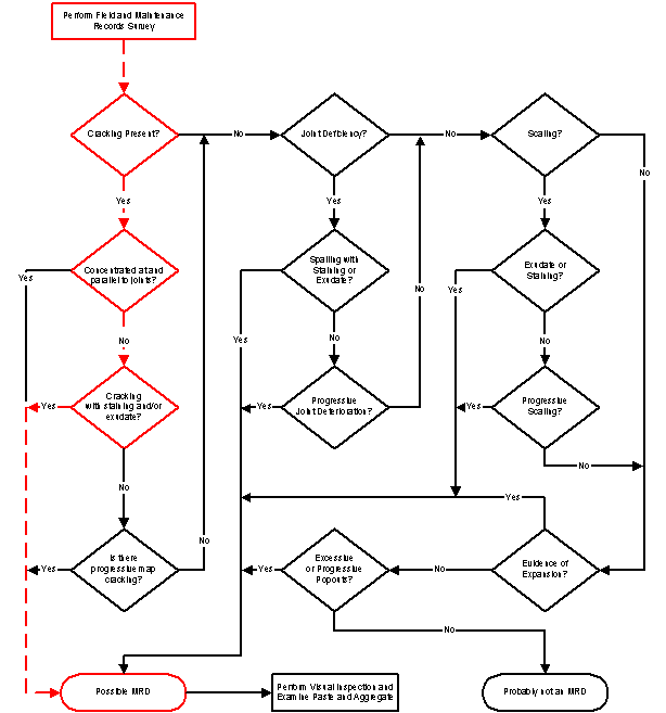
Having performed the described laboratory analyses and applied the diagnostic flowcharts as shown in figures 3-16 through 3-20, several possible MRDs were identified in SD-090-019-001, including ASR, ACR, aggregate freeze-thaw, and deicer attack. This is consistent with the visual observations of the distress reported from the field where mixtures of diagnostic features were apparent. To finalize the diagnosis, the diagnostic tables were consulted. The diagnostic features identified in the analysis processes are listed below in table 3-9 along with their associated MRD type and significance as related to this pavement. A brief discussion follows of each possible MRD identified in the laboratory analysis:
ASR - This MRD seems to be the most dominant given its extent in the sections sampled. From the standpoint of the guidelines, all diagnostic features of ASR were present with the exception of known poor performance for the aggregate used.
ACR - This MRD was identified as a possible but in the final analysis is not listed as probable as a major contributor. Although there was strong evidence of the reactivity of some dolomite aggregates, the extent and magnitude of this reaction was not great.
Aggregate Freeze-Thaw - Like ASR, this appeared to be a dominant distress in terms of extent. The likelihood or certainty of diagnosis is also very high given that, with the exception of known poor performance for the aggregate used, 75 percent of all diagnostic features for aggregate freeze-thaw were present.
Deicer Attack - This MRD is probably the most difficult to diagnose as it can often be present and hidden by other MRDs. The key diagnostic feature that makes deicer attack probable is the occurrence of hydrocalumite as an infilling material in cracks and voids.
As stated previously, it is not rare to find a pavement with diagnostic features representative of more than one distress mechanism present. In most of these cases, as with this one, the failure of the concrete cannot be attributed to one particular cause. However, in this case some general observations can be made. First, the ASR, aggregate freeze-thaw, and potential ACR distresses may not have occurred if a higher quality aggregate source was used. As is most often the case, contractors use the best possible aggregate source economically feasible but in some locations, such as central South Dakota, the possibilities are limited. The other distress mechanism identified, deicer attack, is more problematic as deicers are clearly required on this portion of the interstate system. A lower water-to-cement ratio (w/c) would likely reduce the concrete permeability and thus reduce the likelihood of a recurrence of this distress.
Using the procedures presented in Guideline III in Volume 2: Guidelines Description and Uses, feasible treatment and rehabilitation alternatives were selected. The two most significant MRD mechanisms found were aggregate freeze-thaw deterioration and ASR. Because the two mechanisms are acting in concert, it is difficult to rate the severity of each independently, but the level of spalling and patching at the transverse joints indicates that the severity level is likely a medium severity in Section 001 and medium to high in Section 002. The extent was at both joints and cracks and at corners. As a result, feasible treatment/rehabilitation alternatives include:
The use of patching is still feasible even though ASR was observed since most deterioration is isolated in the vicinity of joints and cracks. Further, lithium compounds are not suggested since they are ineffective in delaying aggregate freeze-thaw damage.
Ultimately, as the pavement continues to deteriorate,
a reconstruction/recycling option becomes more viable. If recycling is considered,
precautions must be taken to avoid aggregate freeze-thaw deterioration and/or
ASR in the newly constructed pavement.
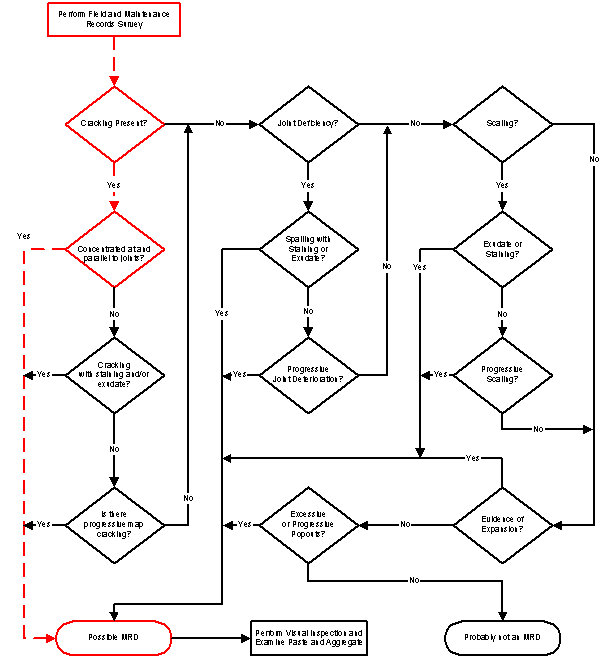
Figure 3-16. Flowchart for assessing the likelihood of MRD causing the observed distress in the pavement as applied to the Spearfish, South Dakota site.
|
Possible Distress |
Present |
Additional Information |
|
|---|---|---|---|
|
Error in Mix Proportioning |
Yes |
No |
See Recommended Literature |
|
Poor Placement |
Yes |
No |
See Recommended Literature |
|
Poor Finishing/Curing |
Yes |
No |
See Recommended Literature |
|
Poor Steel Placement |
Yes |
No |
See Recommended Literature |
|
Carbonation at Depths > 5-10 mm |
Yes |
No |
See Recommended Literature |

Figure 3-17. Flowchart for assessing general concrete properties based on visual examination as applied to the Spearfish, South Dakota site.
Figure 3-18. Flowchart for assessing the condition of the concrete paste as applied to the Spearfish, South Dakota site.
|
Possible Distress |
Present |
Additional Information |
|
|---|---|---|---|
|
Natural Cracking of Aggregate |
Yes |
No |
See Recommended Literature |
|
Sample Preparation Cracks |
Yes |
No |
See Recommended Literature |
|
Aggregate Freeze Thaw |
Yes |
No |
Table II-3 |
|
Natural Weathering of Aggregates |
Yes |
No |
See Recommended Literature |
|
Alkali Silica Reaction |
Yes |
No |
Table II-6 |
|
Alkali Carbonate Reaction |
Yes |
No |
Table II-7 |
|
Secondary Deposits |
Yes |
No |
Figure 3-20 |
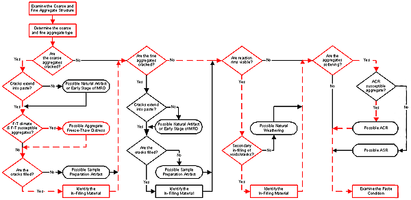
Figure 3-19. Flowchart for assessing the condition of the concrete aggregates as applied to the Spearfish, South Dakota site.
|
Possible Distress |
Present |
Additional Information |
|
|---|---|---|---|
|
Sulfate Attack |
Yes |
No |
Table II-4 |
|
Deicer Attack |
Yes |
No |
Table II-5 |
|
Alkali Silica Reaction |
Yes |
No |
Table II-6 |
|
Alkali Carbonate Reaction |
Yes |
No |
Table II-7 |
|
Corrosion of Embedded Steel |
Yes |
No |
Table II-1 |
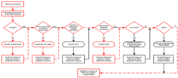
Figure 3-20. Flowchart for identifying infilling materials in cracks and voids as applied to the Spearfish, South Dakota site.
Table 3-9. Identified diagnostic features along with their associated MRD type and significance as related to SD-090-019.
|
Diagnostic |
Method of Characterization |
Associated with MRD Type |
Significance |
|---|---|---|---|
|
Secondary deposits filling air voids |
Staining |
Paste freeze-thaw, deicer attack, ASR, ACR, Sulfate attack (both internal and external) |
Low |
|
Staining at joints or cracks |
Field evaluation |
Deicer attack |
Moderate |
|
Secondary deposits of chloroaluminates |
Petrographic OM |
High |
|
|
Cracking near joints/cracks |
Field evaluation |
Aggregate freeze-thaw |
Moderate |
|
Staining/Spalling |
Field evaluation |
Moderate |
|
|
Cracks through non-reactive coarse aggregates |
Visual inspection |
High |
|
|
Poor void structure in the aggregate |
Petrographic OM |
High |
|
|
Map Cracking with exudate |
Visual inspection |
ASR |
High |
|
ASR reaction product in cracks and voids |
Stereo OM |
High |
|
|
Reaction rims on aggregates |
Visual inspection |
Moderate |
|
|
Microcracking radiating from reacted cracked aggregate |
Stereo OM |
High |
|
|
Map Cracking |
Field evaluation |
Sulfate attack |
Moderate |
|
Significant sulfate deposits in cracks and voids |
Staining |
Low |
For the distresses noted, the best preventative strategy is to use a different source of aggregate. Testing in accordance with the guidelines should show that the current source would be unacceptable without mitigation. Mitigation strategies for aggregate freeze-thaw deterioration that could be used if current aggregate source is all that is available include:
To address the potential for ASR, the following strategies can be employed to reduce the reactivity of the aggregate:
If aggregate benefaction is not feasible or cost effective, other strategies can also be employed including:
Regardless of the approach, the design PCC mixture must be tested to ensure that the aggregate freeze-thaw deterioration and ASR have been mitigated.
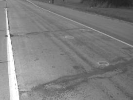
The Minnesota DOT provided several candidate projects with durability problems. One of the projects-located on TH 65 in downtown Mora-was experiencing severe durability problems concentrated at the transverse joints. This project was selected as the primary case study site for the wet-freeze climatic region. This area receives approximately 660 mm of annual precipitation and has a freezing index of 1030 °C-days.
Table 3-10 presents a summary of the design information for this project. This project extends from milepost 64.2 to 65.0 and is located in both the northbound and southbound lanes. It is a four-lane divided roadway separated by a concrete median; some sections also include an additional lane for left-turn traffic. The pavement, which was constructed in 1989, consists of a 200-mm jointed plain concrete pavement (JPCP) with a 75-mm granular base and a 305-mm granular subbase. The transverse joints are skewed and have a variable joint spacing pattern of 4.0-4.6-5.2-4.6 m. Load transfer is provided by aggregate interlock only; no additional load transfer devices have been employed. The only variation in the two sections is the transverse joint sealant-Section 001 uses silicone sealant and Section 002 uses hot-pour sealant. The longitudinal joints are not sealed. A 2.4-m-wide AC shoulder is placed at the outer edge; there is no inside shoulder due to the concrete median.
Table 3-10. Summary of design features for MN-065-064.
|
Category |
Design Feature |
Description |
|---|---|---|
|
General Information |
Project limits |
MP 64.2 - 65.0 |
|
Highway type |
Divided |
|
|
Number of lanes |
4 |
|
|
Direction |
Northbound/southbound |
|
|
Construction date |
1989 |
|
|
Cumulative ESALs |
~300,000 |
|
|
Pavement |
Pavement type |
JPCP |
|
PCC slab thickness |
200 mm |
|
|
Base |
75-mm granular |
|
|
Subbase |
305-mm granular |
|
|
Subgrade type |
Unknown |
|
|
Transverse |
Joint spacing |
4.0-4.6-5.2-4.6 m |
|
Joint skew |
1:12 |
|
|
Load transfer |
Aggregate interlock |
|
|
Sealant type |
Silicone (001); hot-pour (002) |
|
|
Longitudinal |
Load transfer |
|
|
Sealant type |
None |
|
|
Outer |
Surface type |
AC |
|
Width |
2.4 m |
|
|
Inner |
Surface type |
n/a |
|
Width |
n/a |
|
|
Climatic Conditions |
Region |
Dry-freeze |
|
Annual precipitation1 |
660 mm |
|
|
Freezing index1 |
1030 °C-days |
1 Climatic data are for Minneapolis, Minnesota.
Although the design and construction details are the same, the initial investigation revealed that the southbound lanes were in better condition than the northbound lanes. Thus, two sections were selected for survey, one in each direction. Section 001 is located in the northbound outer lane beginning at milepost 64.6, and Section 002 is located in the southbound outer lane beginning at milepost 64.4. Both sections are constructed at grade. Tables 3-11 and 3-12 provide a summary of the distress survey results for Sections 001 and 002, respectively.
As previously mentioned, Section 001 is exhibiting the worst performance, with most of the deterioration limited to the transverse joints. Joint spalling and bituminous patching are predominant along the transverse joints. The spalling appears to be materials-related and progressed to medium severity in most cases. In some cases, the surface has scaled off and aggregate particles have been exposed. Every transverse joint has been patched over a portion of its length to help address the spalling problem. In fact, the transverse joints were so deteriorated that faulting could not be measured. In addition, maintenance forces on hand during the surveys indicated that removal of the material during the patching operation often extended through the entire depth of the slab. The only other distress noted was a longitudinal crack that extended the length of one slab.
Table 3-11. Summary of pavement condition surveys for MN-065-064-001.
|
Distress Type |
Distress Measure |
Severity Level |
Comments |
|||
|---|---|---|---|---|---|---|
|
Low |
Moderate |
High |
||||
|
Cracking |
Corner Breaks |
number |
0 |
0 |
0 |
|
|
Longitudinal Cracking |
linear meters |
3.5 |
0.0 |
0.0 |
||
|
Transverse Cracking |
number of cracks |
0 |
0 |
0 |
||
|
linear meters |
0.0 |
0.0 |
0.0 |
|||
|
percent of slabs |
0 |
|||||
|
Transverse Joints |
Sealant |
fair to good condition |
silicone sealant |
|||
|
Spalling |
number |
1 |
7 |
0 |
||
|
linear meters |
0.4 |
2.7 |
0 |
|||
|
Faulting |
millimeters |
n/a |
||||
|
millimeters |
n/a1 |
|||||
|
Width |
millimeters |
9.4 |
||||
|
Long. Joints |
Sealant |
n/a |
not sealed |
|||
|
Spalling |
linear meters |
0.0 |
0.0 |
0.0 |
||
|
Shoulder Dropoff |
millimeters |
0.0 |
||||
|
Surface Conditions |
Map Cracking |
number of slabs |
0 |
|||
|
square meters |
0.0 |
|||||
|
Scaling |
number of slabs |
0 |
||||
|
square meters |
0.0 |
|||||
|
Polished Aggregate |
square meters |
0.0 |
||||
|
Popouts |
number/sq. meter |
0.0 |
||||
|
Other |
Blowups |
number |
0 |
|||
|
Flexible Patches |
number |
0 |
33 |
0 |
||
|
square meters |
0.0 |
28.3 |
0.0 |
|||
|
Rigid Patches |
number |
0 |
0 |
0 |
||
|
square meters |
0.0 |
0.0 |
0.0 |
|||
|
Pumping/Bleeding |
number |
0 |
||||
|
linear meters |
0.0 |
|||||
1 Faulting could not be measured due to deterioration at transverse joints.
Section 002 is in better overall condition but still exhibits some deterioration at the transverse joints. Medium-severity spalling is observed at 6 of the 33 joints (18 percent) and bituminous patches are observed at 12 of the 33 joints (36 percent). However, the deterioration at the affected joints is less severe than that observed on Section 001. Faulting could be measured on this section and averaged 2.0 and 1.7 mm at 0.30 and 0.75 m from the outer slab edge. The only other distresses include a single transverse crack and a single longitudinal crack.
A more detailed evaluation of the attributes of the MRDs was also conducted in the field. Table 3-13 provides the results of this characterization. Figure 3-21 shows some typical distress manifestations. Although a definitive diagnosis should not be drawn from this evaluation, it does provide information that can help diagnose the distress in conjunction with the laboratory results.
Table 3-12. Summary of pavement condition surveys for MN-065-064-002.
|
Distress Type |
Distress |
Severity Level |
Comments |
|||
|
Low |
Moderate |
High |
||||
|
Cracking |
Corner Breaks |
number |
0 |
0 |
0 |
|
|---|---|---|---|---|---|---|
|
Longitudinal Cracking |
linear meters |
0.0 |
2.7 |
0.0 |
||
|
Transverse Cracking |
number of cracks |
1 |
0 |
0 |
||
|
linear meters |
4.3 |
0.0 |
0.0 |
|||
|
percent of slabs |
3 |
|||||
|
Transverse Joints |
Sealant |
fair condition |
hot-pour sealant |
|||
|
Spalling |
number |
0 |
6 |
0 |
||
|
linear meters |
0.0 |
3.3 |
0.0 |
|||
|
Faulting |
millimeters |
2.0 |
measured at 0.30 m |
|||
|
millimeters |
1.7 |
measured at 0.75 m |
||||
|
Width |
millimeters |
15.7 |
||||
|
Long. Joints |
Sealant |
n/a |
not sealed |
|||
|
Spalling |
linear meters |
0.0 |
0.0 |
0.0 |
||
|
Shoulder Dropoff |
millimeters |
0.0 |
||||
|
Surface Conditions |
Map Cracking |
number of slabs |
0 |
all slabs affected |
||
|
square meters |
0.0 |
entire area |
||||
|
Scaling |
number of slabs |
0 |
||||
|
square meters |
0.0 |
|||||
|
Polished Aggregate |
square meters |
0.0 |
||||
|
Popouts |
number/sq. meter |
0.0 |
||||
|
Other |
Blowups |
number |
0 |
|||
|
Flexible Patches |
number |
0 |
12 |
0 |
||
|
square meters |
0.0 |
7.0 |
0.0 |
|||
|
Rigid Patches |
number |
0 |
0 |
0 |
||
|
square meters |
0.0 |
0.0 |
0.0 |
|||
|
Pumping/Bleeding |
number |
0 |
||||
|
linear meters |
0.0 |
|||||
On both pavement sections, the MRD is confined to the transverse joints; it is not exhibited over the entire slab. The distress is exhibited as hairline cracks that typically run parallel to the transverse joint. The cracking appears to initiate at the transverse joint and progresses outward. As the deterioration progresses, scaling occurs at the surface and exposes the aggregate particles. For the most part, the cracking and deterioration is confined to 150 mm on either side of the joint. The cracks do not have any staining or exudate in or around the cracks.
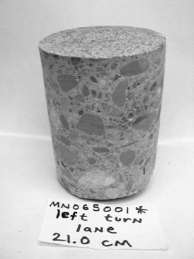
Interestingly, adjacent to Section 001 was a left-turn lane that was part of the original road constructed in the 1950's. This turn-lane appeared to be in excellent condition and it was decided that the turn-lane should also be sampled, thereby providing an insight into a concrete pavement from the same environment, made from similar materials that performed well.
Table 3-13. Summary of MRD characterization for MN-065-064.
|
Description |
Section 001 |
Section 002 |
Comments |
|
|
Cracking |
Location |
Joints |
Joints |
Assumed on spalled joints |
|---|---|---|---|---|
|
Orientation/shape |
Parallel to transverse joints |
Parallel to transverse joints |
Assumed on spalled joints |
|
|
Extent |
Within 150 mm of joint |
Within 150 mm of joint |
||
|
Crack size |
Hairline |
Hairline |
||
|
Staining |
Location |
None |
None |
|
|
Color |
n/a |
n/a |
||
|
Exudate |
Present |
None |
None |
|
|
Color |
n/a |
n/a |
||
|
Extent |
n/a |
n/a |
||
|
Scaling |
Location |
None |
None |
|
|
Area of surface |
n/a |
n/a |
||
|
Depth |
n/a |
n/a |
||
|
Vibrator Trails |
Visible |
None |
None |
|
|
Discolored |
n/a |
n/a |
||
|
Distressed |
n/a |
n/a |
||
|
Change in texture |
n/a |
n/a |
||
|
|
|
|
(a) |
(b) |
Figure 3-21. Typical distress manifestations observed at MN-065-064.
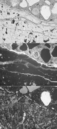
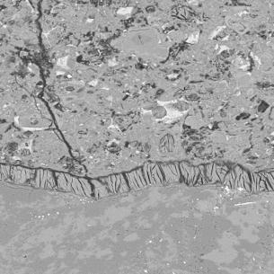
Core Selection/Visual Inspection
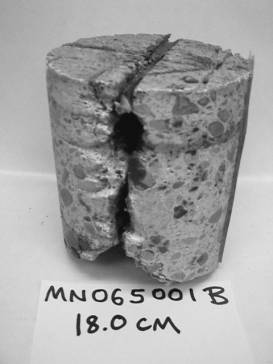
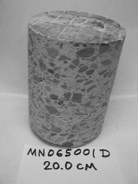
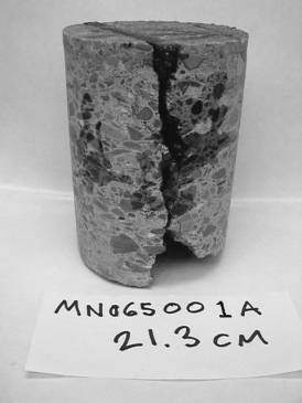
Based on the field survey and site inspection by researchers, the distress was determined to be concentrated at the transverse joints. In addition, the northbound turning lane was recognized as being in good condition even though it was approximately 40 years older than the badly distressed northbound Section 001. The guidelines for sampling were applied and four cores were retrieved from each section. Also, one mid-panel core (core D in standard pattern) was retrieved from the northbound (Section 001) left-turn lane. The cores selected for laboratory analysis were A from Section 002, cores B and D from Section 001, and core D from the left-turn lane. Pictures of these cores are shown in figure 3-22.
Inspecting the cores visually before and after slicing, mix proportions were only noted. If required to understand the distress, an estimate of the relative phase abundance is obtained simultaneously with determination of the hardened air content. The concrete was well consolidated with no apparent segregation or parallelism of the aggregates. Scaling was present in the deteriorated areas but not on the cores examined. Also, no evidence of sub-parallel cracking was apparent on these cores, no entrapped water voids were seen under aggregates, and no surface cracking was seen in the cores. In the mid-panel core D from Section 001, abundant infilling of the entrained air voids was seen and the paste appeared "soft." The mid-panel core from the left-turn lane also had abundant air void infilling but had a much harder paste. Also, the turn-lane concrete had a coarse aggregate that was not crushed and had a larger (25.4 mm) top size. This is in contrast to the concrete in Section 001, which used a crushed aggregate with a 19-mm top size. The concrete at the joint and in contact with the subbase had a depth of carbonation of 5-10 mm. This indicates some deterioration of the paste at those locations.
Stereo Optical Microscopy/Staining Tests
The rock type for the coarse aggregate was characterized as varying, but was dominantly mafic rock types typical of the Superior Lobe. The fine aggregate was the same, but with more quartz. No unusual alteration of the aggregate was observed. For this study, the most useful role for the stereo microscope was for observing stained specimens and determination of the hardened air content. The barium chloride/potassium permanganate stain described in Guideline II colors sulfate minerals a brilliant pink to purple hue as shown in figure 3-23.
Hardened Air-Void Analysis According to ASTM C 457
The hardened air-void content was determined in accordance with ASTM C 457. For the work performed in this study, the modified point count method was used for analysis and the required software was written in house using the free image analysis program from NIST Image 1.62. The results of the analysis are presented in table 3-14.
Table 3-14. Results of ASTM C 457 on concrete from MN-065-064-001.
|
Original |
Existing |
Volume Percent |
|||||
|---|---|---|---|---|---|---|---|
|
Core |
Air |
Spacing Factor |
Air |
Spacing Factor |
Paste |
Coarse |
Fine |
|
Site 1 Core C |
5.9 |
0.227 |
5.9 |
.270 |
26.4 |
39.2 |
28.5 |
|
Site 1 Core B |
3.6 |
.271 |
3.5 |
.302 |
32.4 |
36.4 |
27.5 |
|
Site 1 Core D |
6.3 |
.302 |
6.2 |
.303 |
30.3 |
42.8 |
20.6 |
|
Left Turn Ln. |
4.5 |
.191 |
4.4 |
.220 |
21.9 |
53.9 |
19.7 |
As can be seen, the original air-void system and the existing air-void system (after infilling) are both inadequate in terms of the Power's spacing factor for each. This indicates a cement paste that is not adequately protected from the cyclic stresses of freezing and thawing. This usually results in cracking of the paste that is then susceptible to ingress of water and deicers.
|
|
|
|
(a) |
(b) |
|
|
|
|
(c) |
(d) |
Figure 3-22. Cores evaluated for MN-065-064.
|
|
|
Figure 3-23. Stereo optical micrographs showing sulfate minerals filling air voids.
Petrographic Optical Microscopy
Petrographic microscopy was used to further examine the infilling material present in the air voids. In addition to ettringite, which was common, hydrocalumite (Friedel's Salt) was also identified. The hydrocalumite was most common in the concrete in contact with the subbase. There appeared to be little difference between the cores from the joint and from the mid-panel of Section 001. In general, there was extensive infilling of voids and the cement paste appeared to be very porous and soft. Therefore, in addition to identifying infilling material within voids and cracks, epifluorescent techniques were used for examining the cement paste in the mid-panel cores from Section 001 and the left-turn lane of the northbound section. This analysis leads to an estimate of the w/c ratio for the concrete.
The technique used is commonly known as the UV dye method for determining w/c and uses a fluorescent dye epoxy impregnation preparation and microscopic observation using UV illumination. This method of w/c determination relies upon the relationship between measurements of cement paste fluorescence and the w/c values of known concrete standards (Mayfield 1990; Elsen et al. 1995; Jakobsen et al. 1997). To determine the w/c of a sample of concrete, fluorescence measurements are made from the cement paste, and related back to fluorescence measurements from the concrete standards. The intensity of the fluorescence measurements depends upon the amount of dyed epoxy absorbed by the cement paste. Cement pastes of higher w/c absorb more of the dyed epoxy because they possess a larger volume of capillary porosity than do cement pastes of lower w/c.
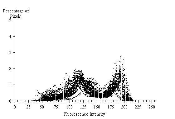
To measure the fluorescence of the cement paste, a concrete thin section is illuminated from above with blue light. The blue light causes the dyed epoxy to fluoresce yellow-green. A blocking filter is used remove the blue light reflected from the surface, allowing only the yellow-green fluorescence to reach the camera (Walker 1992). The camera generates a video signal, which is converted to an RGB digital image on a computer monitor. In the image, each pixel is assigned a 0-255 intensity, where 0 represents pure white (high intensity) and 255 represents pure black (low intensity). The G band of the image contains the most information about the fluorescence, and is used to make the cement paste fluorescence measurement.
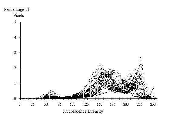
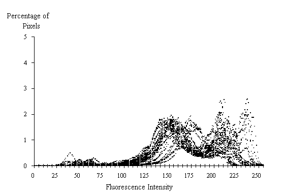
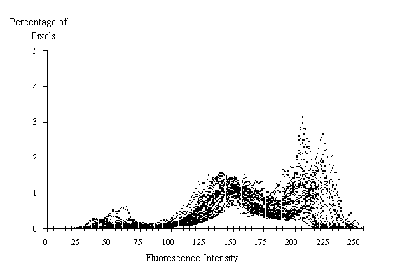
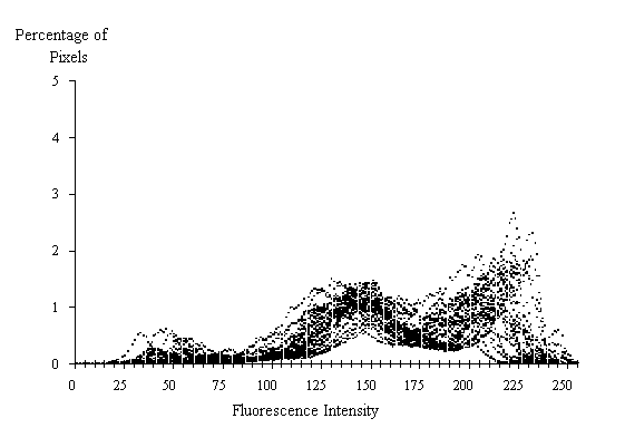
To ensure that the illumination of the blue light and the performance of the camera are constant, a method of calibration is needed. Prior to collecting any measurements, a thin section composed of quartz sand in a matrix of dyed epoxy is used to calibrate the system. A digital image of the calibration slide is collected. In the image, the quartz sand appears dark, and the dyed epoxy matrix appears bright. If a histogram is plotted of the image, two distinct peaks are present, one for the quartz sand, and the other for the dyed epoxy matrix. It is important that the positions of the peaks on the x-axis do not shift in order to ensure consistent measurements. Figure 3-24 shows a summary of histograms collected from our calibration thin section. If the peak positions are out of alignment, then adjustments need to be made, either in the illumination, shutter speed of the camera, or gain and offset of the digital capture card. It has been reported that the fluorescence of the dyed epoxy decreases under constant illumination, but recovers to its initial fluorescence if allowed to sit in darkness for a period of 2 hours (Jakobsen et al.1995). Furthermore, the drop-off in fluorescence is most dramatic within the first 2 minutes, so it is important not to pause too long over any given area before collecting a fluorescence measurement.
Another set of parameters that can affect the fluorescence measurements is consistency in thickness of the thin sections, uniformity of impregnation by the dyed epoxy, and the consistency in dosage of dye. It is imperative that the thin sections used are of high quality (Elsen et al. 1995; Jakobsen et al. 1997).
Since concrete is a combination of cement paste, aggregate, and air bubbles, it is necessary to distinguish between the cement paste fluorescence and the fluorescence from aggregates and air bubbles. Generally, the aggregates are less porous than the cement paste, and therefore fluoresce at lower intensity levels, although this may not always be the case, especially when porous aggregates are used. At the other extreme, total porosity, the air bubbles fluoresce at a higher intensity level than the cement paste. At intermediate intensity values, most of the fluorescence can be attributed to the cement paste. Although this is a good approximation, intensity level alone is not enough to determine whether any given pixel represents cement paste, aggregate, or air bubble. Rigorous schemes have been proposed to ensure that the pixels used to make the cement paste fluorescence measurements do not include air bubbles or aggregate, but they were not employed here (Elsen et al. 1995; Gerold 2000). Instead, the distinction between cement paste, aggregate, or air bubble was based solely on fluorescence intensity.
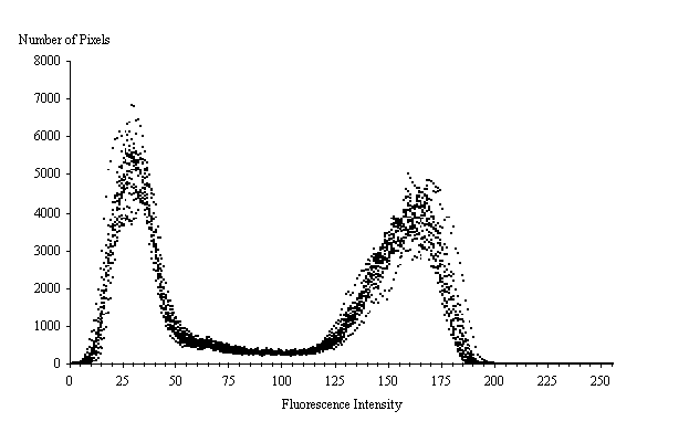
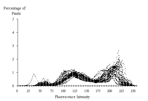
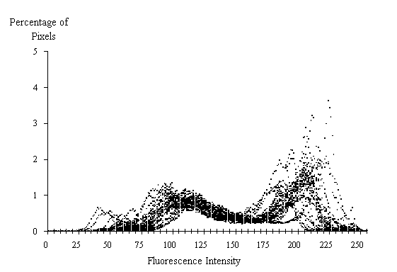
Figures 3-25 through 3-31 summarize the fluorescence measurements from the different standards. Three thin sections were prepared from each w/c standard, and 10 fluorescence measurements were made from different locations on each thin section for a total of 30 measurements per w/c standard. Each fluorescence measurement represents a 2.493-mm x 1.870-mm region on the thin section; therefore, a total area of about 140 mm2 was measured per w/c standard. Each measurement consists of a 640 x 480 pixel image, so a total of 9.216 million pixels were collected per w/c standard. Regions containing coarse aggregates were avoided during the sampling. The regions sampled were chosen by the operator, which may introduce bias.
Figure 3-24. Histogram of 16 fluorescence measurements from calibration thin section composed of quartz sand in a dyed epoxy matrix. The peak on the left represents the dyed epoxy matrix, and the peak on the right represents the quartz sand.
It is clear from figures 3-25 through 3-31 that there is considerable variability within the individual standards, although the three distinct fluorescence levels attributed to air bubbles, cement paste, and aggregate can be distinguished in each of the standards. Assuming that the intermediate intensity levels represent the cement paste, channels 75 through 175 were used to quantify the cement paste fluorescence of the standards. The choice of channels 75 through 175, however, does not ensure that the pixels included in the measurement exclusively represent cement paste, nor does it ensure that some pixels that represent cement paste are not omitted. One concern is that the choice of channels 75 to 175 may exclude unhydrated cement grains, which appear as dark specks against the background of cement hydration products and capillary porosity. The overall fluorescence of the cement paste is related to both the capillary porosity as well as the quantity of unhydrated cement grains. In these measurements, variations in capillary porosity alone seem sufficient to distinguish variations in w/c (see figure 3-32). However, with the inclusion of unhydrated cement grains, the variation in intensity versus w/c would perhaps be more pronounced.
There is no doubt that it would be advantageous to employ a more rigorous method to ensure that only those pixels that represent cement paste are used in the measurements, but the simple method employed here performed adequately. The major weakness in the strict use of channels 75 to 175 is that the fluorescence of the cement paste and aggregates are both influenced to some degree by the fluorescence of the surrounding phases. For instance, the cement paste surrounding air bubbles often appears brighter than the rest of the cement paste due to the
Figure 3-25. Histogram of 30 fluorescence measurements from 0.38 w/c standard.
Figure 3-26. Histogram of 30 fluorescence measurements from 0.41 w/c standard.
Figure 3-27. Histogram of 30 fluorescence measurements from 0.42 w/c standard.
Figure 3-28. Histogram of 30 fluorescence measurements from 0.52 w/c standard.
Figure 3-29. Histogram of 30 fluorescence measurements from 0.56 w/c standard.
Figure 3-30. Histogram of 30 fluorescence measurements from 0.74 w/c standard.
Figure 3-31. Histogram of 30 fluorescence measurements from 0.80 w/c standard.
proximity to the air bubbles. For this reason, some researchers exclude cement paste that neighbors air bubbles from recorded fluorescence measurements (Elsen et al. 1995). Similarly, translucent aggregates, such as quartz, may appear brighter if surrounded by brightly fluorescing cement paste. Depending on the appearance of a series of images, it may be necessary to interactively change the interval of channels that is used to represent the fluorescence of the cement paste. However, this would require the operator to repeatedly make decisions that could introduce bias to the measurements, hence the rigid choice of channels 75 to 175 used here.
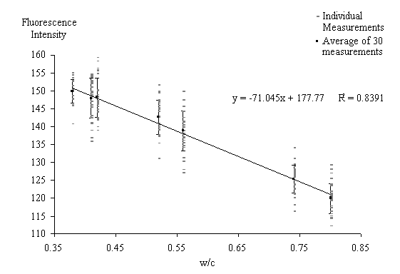
The first step in quantifying the fluorescence for each individual measurement was to normalize the number of pixels contained in channels 75 through 175 to 100. This step is necessary to account for differences in the volumes of cement paste between standards. For instance, the low w/c standards contained a higher volume of cement paste in order to maintain the workability of the plastic concrete. Next, an average intensity value was determined from the normalized number of pixels in channels 75 through 175. The average intensity value was used as a measurement of cement paste fluorescence. Figure 3-32 plots the average fluorescence intensity values versus the w/c of the standards, along with a best-fit line. The equation for the best-fit line from figure 3-32 can then be used to convert average fluorescence intensity measurements from unknown concrete samples to values for w/c.
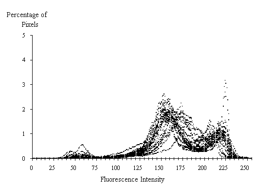
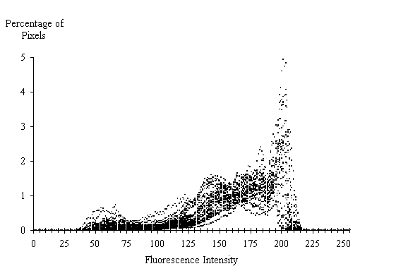
The concrete samples analyzed here are from mid-panel of the traffic lane and from mid-panel of a left-turn lane. Thin sections were prepared from the cores at different depths to make cement paste fluorescence measurements. Figures 3-33 through 3-38 summarize the measurements from the old concrete and the new concrete.
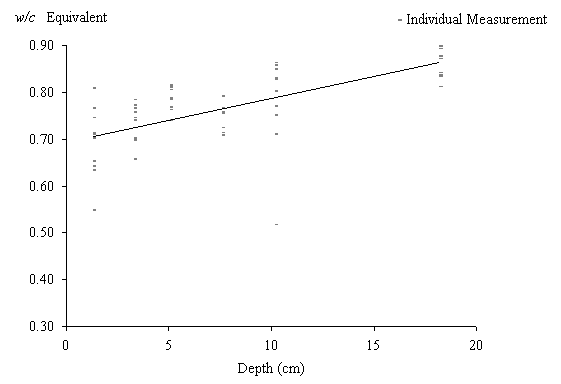
Figure 3-32. Average cement paste fluorescence measurements versus w/c. Error bars represent one standard deviation.
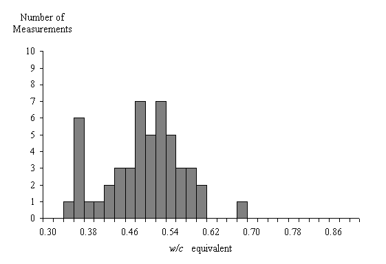
Figure 3-33. Histogram of fluorescence measurements from 1950 concrete from mid-panel of the left-turn lane of site MN-065-064-001.
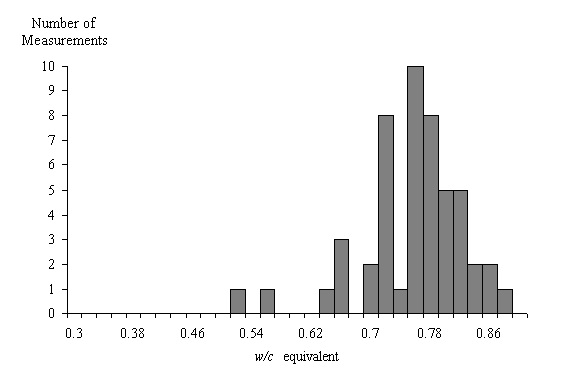
Figure 3-34. Histogram of fluorescence measurements from 1990 concrete from mid-panel of the traffic lane of site MN-065-064-001.
Figure 3-35. Distribution of the w/c values from the 1950 concrete from mid-panel of the left-turn lane of site MN-065-064-001.
Figure 3-36. Distribution of the w/c values from the 1990 concrete from mid-panel of the traffic lane of site MN-065-064-001.
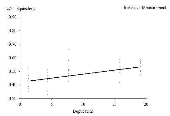
Figure 3-37. The w/c values versus depth from the 1950 concrete from mid-panel of the left-turn lane of site MN-065-064-001.
Figure 3-38. The w/c values versus depth from the 1990 concrete from mid-panel of the traffic lane of site MN-065-064-001.
When using the fluorescent method of w/c determination, it is important to realize that the capillary porosity is not solely a function of the w/c. As both proponents and critics of the technique are quick to point out, the capillary porosity is influenced by a number of different parameters. For example, the degree of hydration, the use of cementitious additives such as fly ash, and the amount of weathering or leaching of the cement paste all influence the capillary porosity, just to name a few (Jakobsen et al. 1997; Neville 1999). Certainly, to make an accurate estimation of w/c, appropriate standards of similar hydration and composition should be used. Since it would be difficult to produce suitable standards for every situation, another approach would be to refer to the fluorescence measurement of w/c as an "equivalent w/c". This makes it clear that the w/c value determined for a sample of concrete is expressed in terms of an equivalent w/c as compared to the standards. In the case of site MN-065-064-001, the w/c standards came from concrete that had cured for 65 days. The concrete from the 1950's has had a long time to hydrate, and it might not be appropriate to directly compare it to the 65-day cure standards. The concrete from 1990 may have undergone some leaching and weathering, so again, it might not be appropriate to directly compare it to the standards as a measure of constructed w/c. However, if it is understood that the w/c measurement is an equivalent to the 65-day cured laboratory standards, then the results are not as misleading.
Scanning Electron Microscopy (SEM)
SEM was used to identify infilling material in voids and cracks. As indicated earlier, the principal materials identified were ettringite and hydrocalumite as shown in the typical SEM micrographs and x-ray analyses presented in figures 3-39 and 3-40.
|
|
|
|---|---|
|
(a) SEM micrograph |
(b) X-ray analysis |
Figure 3-39.Typical SEM micrograph and x-ray analysis for ettringite infilling air void.
|
|
|
|---|---|
|
(a) Hydrocalumite in air void, magnified 716x |
(b) Typical spectrum from hydrocalumite deposit |
Figure 3-40. Typical SEM micrograph and x-ray analysis for hydrocalumite infilling air void.
Table 3-15 presents the quantitative results from a single spectrum collected from an ettringite deposit, compared to a calculated composition for dehydrated ettringite. Table 3-16 is a summary of 10 analyses of hydrocalumite deposits, compared to calculated compositions for the 3 dehydrated end members of the hydrocalumite solid solution series. The ternary diagram presented previously in figure 3-15 shows the probable range of composition for the hydrocalumite deposits analyzed from the pavement. Hydrocalumite describes a solid solution series with 3 end-member compositions and a range in substitutions between Cl-, OH-, and CO32-. The hydrocalumite analyses were low in chlorine as compared to the pure Cl- hydrocalumite end member shown above. Oxygen and carbon were not analyzed so the true composition of the hydrocalumite cannot be determined.
Table 3-15. Quantitative results from single spectrum collected from ettringite deposit, compared to a calculated composition for dehydrated ettringite.
|
Element |
Analysis |
Dehydrated Ettringite (theoretical) |
|---|---|---|
|
Na |
0.0 |
0.0 |
|
Mg |
0.0 |
0.0 |
|
Al |
7.5 |
6.9 |
|
Si |
0.2 |
0.0 |
|
S |
13.0 |
12.2 |
|
Cl |
0.0 |
0.0 |
|
K |
0.0 |
0.0 |
|
Ca |
31.9 |
30.6 |
|
Ti |
0.0 |
0.0 |
|
Mn |
0.0 |
0.0 |
|
Fe |
0.0 |
0.0 |
|
O |
Not Measured |
48.8 |
|
H |
Not Measured |
1.5 |
|
sum |
52.8 |
100.0 |
This test site illustrates a key point with the laboratory analysis of MRD. Namely, standard procedures will provide adequate data for diagnosing the majority of MRD cases. But in some cases, a more in-depth or "unique" analysis must be conducted to fully understand the MRD mechanisms identified. In this case, a more in-depth investigation of the effective w/c led to a better insight into why the distresses observed were occurring.
In the context of a guideline, it is impossible to design an analytical approach that will identify all possible types of MRD in every situation. For more difficult or complex cases of MRD, a State highway agency (SHA) may have to contract with outside labs for petrographic services if such services are not available within the organization. Even if an outside contract is required, the guidelines still assist the analyst or engineer in refining the questions that you want the external petrographer to answer.
Table 3-16. Summary of 10 analyses and theoretical composition of hydrocalumite deposits.
|
Element |
Measured |
Theoretical |
|||
|---|---|---|---|---|---|
|
Average Wt% |
Standard Deviation |
Dehydrated |
Dehydrated |
Dehydrated |
|
|
Na |
0.0 |
0.0 |
0.0 |
0.0 |
0.0 |
|
Mg |
0.0 |
0.0 |
0.0 |
0.0 |
0.0 |
|
Al |
13.2 |
0.3 |
11.0 |
12.9 |
12.5 |
|
Si |
0.0 |
0.0 |
0.0 |
0.0 |
0.0 |
|
S |
0.0 |
0.0 |
0.0 |
0.0 |
0.0 |
|
Cl |
6.6 |
0.4 |
14.5 |
0.0 |
0.0 |
|
K |
0.0 |
0.0 |
0.0 |
0.0 |
0.0 |
|
Ca |
37.2 |
0.5 |
32.8 |
38.3 |
37.3 |
|
Ti |
0.0 |
0.0 |
0.0 |
0.0 |
0.0 |
|
Mn |
0.0 |
0.0 |
0.0 |
0.0 |
0.0 |
|
Fe |
0.5 |
0.1 |
0.0 |
0.0 |
0.0 |
|
C |
Not Measured |
0.0 |
0.0 |
2.8 |
|
|
O |
Not Measured |
39.2 |
45.9 |
44.6 |
|
|
H |
Not Measured |
2.5 |
2.9 |
2.8 |
|
|
sum |
57.4 |
100.0 |
100.0 |
100.0 |
|
Having performed the described laboratory analyses and applied the diagnostic flowcharts reproduced in figures 3-41 to 3-45, two possible MRDs were identified in MN-065-064-001, including paste freeze-thaw and deicer attack. To finalize the diagnosis, the diagnostic tables were consulted. The diagnostic features identified in the analysis processes are listed below in table 3-17 along with their associated MRD type and significance as related to this pavement. A brief discussion follows of each possible MRD identified in the laboratory analysis:
Paste Freeze-Thaw - Clearly, there were two distinguishing features of this distressed concrete. The first was the softness and high effective w/c for this concrete. The porous paste was evident even in the mid panel when compared to the passing lane constructed with similar aggregates but approximately 40 years before the failed concrete. Of course, changes in cement characteristics and other factors may be contributors to the observed paste characteristics. However, it is unlikely that these factors would result in a difference of the magnitude seen in these pavement sections. It is most probable that a high w/c contributed to the observed distress. In addition, the original air system was marginal and once infilling occurred; the hardened air system became inadequate to protect the weakened paste.
Deicer Attack - This MRD may be opportunistic or it may be a contributor. Given the degree of distress seen near the joint, it is reasonable to infer that deicer attack was a factor. Also, the presence of hydrocalumite is an indicator that this concrete was exposed to a high chloride environment, given the necessary high chloride concentration required for this phase to precipitate.
Figure 3-41. Flowchart for assessing the likelihood of MRD causing the observed distress in the pavement as applied to MN-065-064.
|
Possible Distress |
Present |
Additional Information |
|
|---|---|---|---|
|
Error in Mix Proportioning |
Yes |
No |
See Recommended Literature |
|
Poor Placement |
Yes |
No |
See Recommended Literature |
|
Poor Finishing/Curing |
Yes |
No |
See Recommended Literature |
|
Poor Steel Placement |
Yes |
No |
See Recommended Literature |
|
Carbonation at Depths > 5-10 mm |
Yes |
No |
See Recommended Literature |
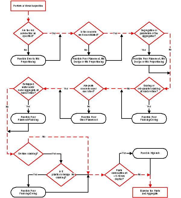
Figure 3-42. Flowchart for assessing general concrete properties based on visual examination as applied to MN-065-064.
|
Possible Distress |
Present |
Additional Information |
|
|---|---|---|---|
|
Shrinkage Cracks or Sample Preparation Cracks |
Yes |
No |
See Recommended Literature |
|
Paste Freeze-Thaw |
Yes |
No |
Table II-2 |
|
Aggregate Freeze-Thaw |
Yes |
No |
Table II-3 |
|
Sulfate Attack |
Yes |
No |
Table II-4 |
|
Deicer Attack |
Yes |
No |
Table II-5 |
|
Secondary Deposits |
Yes |
No |
Figure 3-45 |
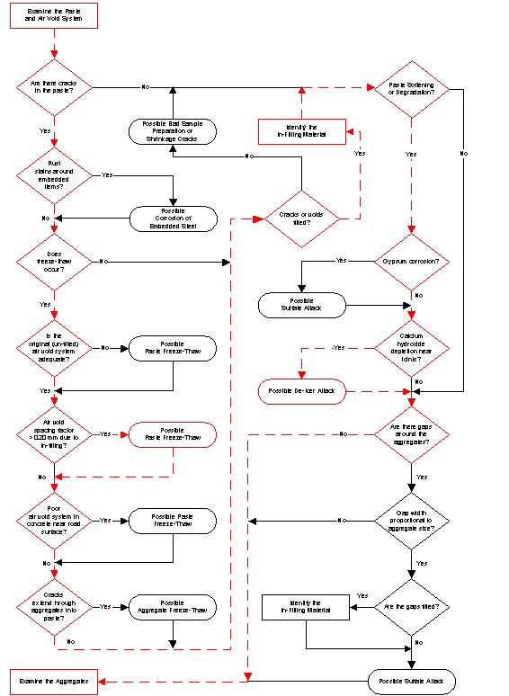
Figure 3-43. Flowchart for assessing the condition of the concrete paste as applied to MN-065-064.
|
Possible Distress |
Present |
Additional Information |
|
|---|---|---|---|
|
Natural Cracking of Aggregate |
Yes |
No |
See Recommended Literature |
|
Sample Preparation Cracks |
Yes |
No |
See Recommended Literature |
|
Aggregate Freeze Thaw |
Yes |
No |
Table II-3 |
|
Natural Weathering of Aggregates |
Yes |
No |
See Recommended Literature |
|
Alkali Silica Reaction |
Yes |
No |
Table II-6 |
|
Alkali Carbonate Reaction |
Yes |
No |
Table II-7 |
|
Secondary Deposits |
Yes |
No |
Figure 3-45 |
Figure 3-44. Flowchart for assessing the condition of the concrete aggregates as applied to MN-065-064.
|
Possible Distress |
Present |
Additional Information |
|
|---|---|---|---|
|
Sulfate Attack |
Yes |
No |
Table II-4 |
|
Deicer Attack |
Yes |
No |
Table II-5 |
|
Alkali-Silica Reaction |
Yes |
No |
Table II-6 |
|
Alkali-Carbonate Reaction |
Yes |
No |
Table II-7 |
| Corrosion of Embedded Steel |
Yes |
No |
Table II-1 |
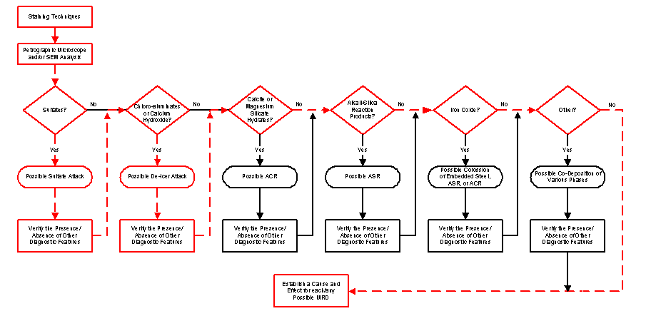
Figure 3-45. Flowchart for identifying infilling materials in cracks and voids as applied to MN-065-064.
Table 3-17. Diagnostic features identified along with their associated MRD type and significance as related to MN-065-064.
|
Diagnostic |
Method of Characterization |
Associated with MRD Type |
Significance |
|---|---|---|---|
|
Secondary deposits filling air voids and cracks |
Visual |
Paste freeze-thaw, deicer attack, sulfate attack (both internal and external) |
Low |
|
Surface scaling or Sub-parallel cracking |
Field evaluation |
Paste freeze-thaw |
Medium-Low |
|
Inadequate air-void system |
Visual |
High |
|
|
Scaling of slab surface |
Field evaluation |
Deicer attack |
Medium |
|
Secondary deposits of chloroaluminates |
Petrographic OM |
High |
|
|
Secondary deposits of ettringite in air voids and cracks |
Petrographic OM |
Sulfate attack |
Low |
In summary, a combination of heavy deicer use, an inadequate air-void system, and a weak paste resulting from a high w/c all combined to cause the distress in this pavement. With care in batching future concrete mixes and possibly alternative deicers, this type of distress may be minimized in future construction.
The application of the procedures presented in Guideline III in Volume 2: Guidelines Description and Uses is not straightforward in this case since the high w/c is a major factor in the observed failure, yet it is not considered a common MRD. Even so, the guideline can be used to select feasible treatment and rehabilitation alternatives for paste freeze-thaw deterioration and deicer attack. Based on the visual assessment, Section 001 is clearly suffering high-severity distress in the vicinity of joints, with patching observed at every joint. Section 002 is in slightly better condition, but still would be considered high severity based on the depth of spalling and the number of patches observed. It was also noted by maintenance crews that the deterioration extended through the full depth of the slab. Based on this assessment, the following treatment/rehabilitation options are available:
The use of full-depth patching is still feasible, although it should only be used as a stop-gap measure with the full realization that deterioration will likely continue at the patch boundary. Ultimately, as the pavement continues to deteriorate, a reconstruction/recycling option becomes more viable.
For the distresses noted, the best preventative strategy is to ensure that the concrete specified is constructed. It seems evident that the w/c as constructed was well in excess of that specified and that the as-constructed air-void system was inadequate to protect against paste freeze-thaw damage. Further, the deicer attack was also a result of these two factors. If this concrete was constructed as specified, it is unlikely that deterioration would have occurred. Thus, the use of a w/c equal to or less than 0.45 and the addition of an effective air entraining admixture at a dosage sufficient to create an adequate air-void system would be all that was needed to address the observed MRD.
Pavements with durability problems in the wet-nonfreeze climatic region were not as easy to locate. However, the North Carolina DOT did provide a viable section that was selected as the primary site for the wet-nonfreeze region (this area receives approximately 1070 mm of annual precipitation and has a freezing index of 58°C-days). The section is located on I-440 near Raleigh and exhibits surface cracking over the entire slab area. The project extends approximately 3 km from Pool Road to Raleigh Boulevard in both directions. The highway is a divided roadway with a minimum of three and in some cases up to five lanes in each direction.
The project was constructed in 1982 and consists of a 250-mm JPCP and a 100-mm cement-treated base. A 25-mm AC separator layer is located between the PCC slab and the base course. The transverse joints are doweled, sealed with silicone, and employ a variable joint spacing pattern of 7.6-7.0-5.8-5.5 m. The longitudinal joints were formed using a plastic joint insert and have not been sealed. AC shoulders are located along the inside and outside edge and are 1.8 and 3.0 m wide, respectively. The design information is summarized in table 3-18.
An initial windshield survey was conducted over the entire project. Following this cursory survey, two sections-one in each direction-were selected for more detailed surveys. Both sections are located in the outer traffic lane. Table 3-19 presents a summary of the distress survey results for Section 001; the results for Section 002 are summarized in table 3-20.
Both sections are in similar condition. The predominant distress is map cracking over the entire pavement surface. Several flexible patches (low to medium severity) have also been placed on each section. Faulting is not to the extent where it is creating any reduction in ride quality. The only observed difference is the presence of two transverse cracks on Section 002. Due to the surface cracking, these cracks have begun to deteriorate and have been patched with AC. The transverse joints, which have been sealed with a silicone sealant, are in fair condition. However, it appears that as this MRD continues to progress, it could result in problems in the future.
Table 3-18. Summary of design features for NC-440-015.
|
Category |
Design Feature |
Description |
|---|---|---|
|
General |
Project limits |
Pool Road to Raleigh Blvd. |
|
Highway type |
Divided |
|
|
Number of lanes |
6 |
|
|
Direction |
Eastbound/westbound |
|
|
Construction date |
1982 |
|
|
Cumulative ESALs |
||
|
Pavement Cross Section |
Pavement type |
JPCP |
|
PCC slab thickness |
250 mm |
|
|
Base |
100-mm cement-treated base (CTB)1 |
|
|
Subbase |
||
|
Subgrade type |
||
|
Transverse Joint |
Joint spacing |
7.6-7.0-5.8-5.5 m |
|
Joint skew |
None |
|
|
Load transfer |
Dowels |
|
|
Sealant type |
Silicone |
|
|
Longitudinal |
Load transfer |
|
|
Sealant type |
None |
|
|
Outer Shoulder |
Surface type |
AC |
|
Width |
3.0 m |
|
|
Inner Shoulder |
Surface type |
AC |
|
Width |
1.8 m |
|
|
Climatic |
Region |
Wet-nonfreeze |
|
Annual precipitation |
1070 mm |
|
|
Freezing index |
58 °C-days |
1 Also includes 25-mm AC separator layer between the CTB and PCC slab.
Table 3-19. Summary of pavement condition surveys for NC-440-015-001.
|
Distress Type |
Distress Measure |
Severity Level |
Comments |
|||
|---|---|---|---|---|---|---|
|
Low |
Moderate |
High |
||||
|
Cracking |
Corner Breaks |
number |
0 |
0 |
0 |
|
|
Longitudinal Cracking |
linear meters |
0.0 |
0.0 |
0.0 |
||
|
Transverse Cracking |
number of cracks |
0 |
0 |
0 |
||
|
linear meters |
0.0 |
0.0 |
0.0 |
|||
|
percent of slabs |
0 |
|||||
|
Transverse Joints |
Sealant |
fair condition |
silicone sealant |
|||
|
Spalling |
number |
2 |
0 |
0 |
||
|
linear meters |
0.5 |
0.0 |
0 |
|||
|
Faulting |
millimeters |
n/a1 |
||||
|
millimeters |
1.2 |
|||||
|
Width |
millimeters |
8.1 |
||||
|
Long. Joints |
Sealant |
n/a |
not sealed |
|||
|
Spalling |
linear meters |
0.0 |
0.0 |
0.0 |
||
|
Shoulder Dropoff |
millimeters |
n/a |
not measured |
|||
|
Surface Conditions |
Map Cracking |
number of slabs |
24 |
all slabs affected |
||
|
square meters |
578.0 |
entire area |
||||
|
Scaling |
number of slabs |
0 |
||||
|
square meters |
0.0 |
|||||
|
Polished Aggregate |
square meters |
0.0 |
||||
|
Popouts |
number/sq. meter |
0.0 |
||||
|
Other |
Blowups |
number |
0 |
|||
|
Flexible Patches |
number |
5 |
0 |
0 |
||
|
square meters |
0.8 |
0.0 |
0.0 |
|||
|
Rigid Patches |
number |
0 |
0 |
0 |
||
|
square meters |
0.0 |
0.0 |
0.0 |
|||
|
Pumping/Bleeding |
number |
0 |
||||
|
linear meters |
0.0 |
|||||
1 Faulting could not be measured due to high traffic volumes.
Table 3-20. Summary of pavement condition surveys for NC-440-015-002.
|
Distress Type |
Distress |
Severity Level |
Comments |
|||
|---|---|---|---|---|---|---|
|
Low |
Moderate |
High |
||||
|
Cracking |
Corner Breaks |
number |
0 |
0 |
0 |
|
|
Longitudinal Cracking |
linear meters |
0.0 |
0.0 |
0.0 |
||
|
Transverse Cracking |
number of cracks |
2 |
0 |
0 |
||
|
linear meters |
7.4 |
0.0 |
0.0 |
|||
|
percent of slabs |
8 |
|||||
|
Transverse Joints |
Sealant |
fair condition |
silicone sealant |
|||
|
Spalling |
number |
0 |
0 |
0 |
||
|
linear meters |
0.0 |
0.0 |
0.0 |
|||
|
Faulting |
millimeters |
0.6 |
measured at 0.30 m |
|||
|
millimeters |
0.7 |
measured at 0.75 m |
||||
|
Width |
millimeters |
7.6 |
||||
|
Long. Joints |
Sealant |
n/a |
not sealed |
|||
|
Spalling |
linear meters |
0.0 |
0.0 |
0.0 |
||
|
Shoulder Dropoff |
millimeters |
3.0 |
||||
|
Surface Conditions |
Map Cracking |
number of slabs |
24 |
all slabs affected |
||
|
square meters |
576.0 |
entire area |
||||
|
Scaling |
number of slabs |
0 |
||||
|
square meters |
0.0 |
|||||
|
Polished Aggregate |
square meters |
0.0 |
||||
|
Popouts |
number/sq. meter |
0.0 |
||||
|
Other |
Blowups |
number |
0 |
|||
|
Flexible Patches |
number |
0 |
2 |
0 |
||
|
square meters |
0.0 |
0.4 |
0.0 |
|||
|
Rigid Patches |
number |
0 |
0 |
0 |
||
|
square meters |
0.0 |
0.0 |
0.0 |
|||
|
Pumping/Bleeding |
number |
0 |
||||
|
linear meters |
0.0 |
|||||
An evaluation of the MRDs is a key component of this project, so they are thus examined closely in the field. This detailed investigation, along with the comprehensive laboratory investigation, will help diagnose the type and cause of the distresses. The findings from this evaluation are summarized in table 3-21 and typical photos are shown in figure 3-46.
The primary distress, and the reason this section was selected as part of this project, is the extensive surface cracking exhibited over the entire pavement area. These hairline cracks run parallel to the longitudinal joints and are more prevalent near the outer edge of the slab (i.e., near the longitudinal joints). Some cracks are stained immediately around the cracks, which further highlights the presence of the cracks. The staining is typically dark gray areas around the crack; no exudate appears to be present in the cracks.
Table 3-21. Summary of MRD characterization for NC-440-015.
|
Description |
Section 001 |
Section 002 |
Comments |
|
|---|---|---|---|---|
|
Cracking |
Location |
Entire slab |
Entire slab |
|
|
Orientation/shape |
Parallel to longitudinal joint |
Parallel to longitudinal joints |
||
|
Extent |
Entire slab |
Entire slab |
||
|
Crack size |
Hairline |
Hairline |
||
|
Staining |
Location |
Around cracks |
Around cracks |
Not all cracks have staining |
|
Color |
Dark gray |
Dark gray |
||
|
Exudate |
Present |
None |
None |
|
|
Color |
n/a |
n/a |
||
|
Extent |
n/a |
n/a |
||
|
Scaling |
Location |
None |
None |
|
|
Area of surface |
n/a |
n/a |
||
|
Depth |
n/a |
n/a |
||
|
Vibrator Trails |
Visible |
None |
None |
|
|
Discolored |
n/a |
n/a |
||
|
Distressed |
n/a |
n/a |
||
|
Change in texture |
n/a |
n/a |
||
|
|
|
|
(a) |
(b) |
Figure 3-46. Typical cracking pattern at NC-444-015. Note distress over entire slab length with spalling occuring at joints.
For the most part, these surface cracks are not causing any immediate concerns or problems. At a few joints and at the two transverse cracks, the surface cracks have begun to deteriorate and create loose pieces and some large spalls were seen on the side of the road. These areas have been patched with AC. Otherwise, the cracks are not adversely affecting the ride quality.
Core Selection/Visual Inspection
Based on the field survey and site inspection by researchers, the distress was determined to be widespread and uniform. Therefore it wasn't necessary to emphasize the joints as compared to the mid-panel concrete in selecting cores to analyze. As a result only two cores were examined, cores A and E. In addition, a large spall found by the side of Site 1 was selected for examination. Pictures of the cores and spall are shown in figure 3-47.
Figure 3-47. Cores and specimens evaluated from NC-440-015.
As with the other sites, mix proportions were not documented in the construction records and were only noted in the visual inspection as being normal. The concrete cores were 265 mm in depth, considerably greater than the design thickness of 250 mm. The concrete was well consolidated with no apparent segregation or parallelism of the aggregates. No scaling was present and there was no evidence of sub-parallel cracking or entrapped water voids under aggregates and surface cracking was seen in the cores that was thought not to be shrinkage cracks. Cracks extended from aggregates and through the paste. Secondary deposits were seen in some entrapped air voids and darkened rims were seen on coarse aggregate particles.
As with the other sites, the stereo optical microscope was used to inspect the concrete in greater detail and perform the ASTM C 457 analysis. Infilling in cracks and voids was common with some entrapped air voids exhibiting large amounts of gel products. Figure 3-48 shows examples of infilling. The aggregate shown stained in figure 3-48 was prepared in thin section for additional study. Coarse aggregates in contact with the cement paste showed darkened rims.
|
|
|
|---|---|
|
(a) Desiccated ASR gel lining large entrapped air void. |
(b) Granite coarse aggregate that picked up the stain, especially in cracks within the aggregate. Matching face from this aggregate prepared in thin section to examine material in cracks. |
Figure 3-48. Stereo optical micrographs of ASR gel and reactive coarse aggregate from NC-440-015.
The coarse aggregate type was identified as granite and the fine aggregate appeared to be the same rock type. The fine aggregate was very angular, further indicating it may be a crushed version of the coarse aggregate used. The paste was hard and varied in color from yellow on one site to green on the other. This was attributed to different cement types being used in different sections, a fact later confirmed by observation of the unhydrated cement grains in the concrete using the petrographic optical microscope.
The results of ASTM C 457 are shown below in table 3-22. Both the air-void parameters and phase abundance results are presented. As can be seen, the value of Power's spacing factor measured for this concrete exceeds the maximum recommended to ensure freeze-thaw protection. In general this is not a concern for this pavement as the environment is considered a wet/no-freeze zone. However, the fact is that some freezing does occur and there may be some minor contribution of paste freeze-thaw damage to the overall observed distress.
Table 3-22. Results of ASTM C 457 on concrete from NC-440-015.
|
Original |
Existing |
Volume Percent |
|||||
|---|---|---|---|---|---|---|---|
|
Core |
Air Content |
Spacing Factor |
Air Content |
Spacing Factor |
Paste |
Coarse Aggregate |
Fine Aggregate |
|
Site 1 Core A |
6.6 |
.278 |
6.4 |
.320 |
29.6 |
41.7 |
22.2 |
|
Site 1 Core E |
6.5 |
.252 |
6.5 |
.276 |
30.0 |
44.4 |
21.2 |
The results of staining indicate that both sulfate minerals and ASR gel are present as infilling material in cracks and voids. Figure 3-49 below shows some typical results for these tests. The characteristic yellow of the sodium cobaltinitrite stain is seen on the left and the brilliant purple color associated with the barium chloride/potassium permanganate is seen on the right. The phenolphthalein stain indicated a depth of carbonation of approximately 5 mm at the road surface and at the bottom of the slab.
Figure 3-49. Typical stereo optical micrographs of stained concrete. Note that the broad banding occurs from the montage process to create a single image.
Petrographic Optical Microscopy
The petrographic microscope further confirmed dense reaction rims on coarse aggregates in contact with the cement paste. Cracks within the aggregate were filled with crystalline ASR product and ettringite. The ettringite was generally very dense and tightly packed. In addition to the granite aggregates reacting, some reactive chert was seen in the fine aggregate. Also, the fine aggregate contained some reactive particles that were a red to tan color and occurred as a "coating" on other particles. The reaction seems to convert the coating to a gel product, which appears desiccated in thin section. Apart from consuming the tan to red coating, the reaction appears to cause no damage to the surrounding concrete. Some typical petrographic optical micrographs of reacting aggregate and ASR gel "blobs" are shown in figures 3-50 through 3-54.
Figure 3-50. Petrographic micrographs from spall obtained from NC-440-015 showing ettringite filled entrained air voids. Ettringite growths are unusually dense.
Figure 3-51. Petrogrpahic micrograph of a tan to red coating observed on some of the fine aggregates that appears to undergo ASR from spall obtained from NC-440-015.
Figure 3-52. Petrographic micrograph of ettringite and "ASR gel blob" from spall obtained from NC-440-015. The term ASR gel is misleading in this example, since the reaction product is slightly birefringent and, therefore, crystalline.
Figure 3-53. Petrographic micrograph of ettringite intermixed with ASR gel. As in figure 3-52, the ASR "gel" in this image is birefringent and crystalline.
Figure 3-54. Petrographic micrograph of ASR gel in crack within coarse aggregate. The gel deposit in this image was analyzed with the SEM. Again, the ASR "gel" in this image is birefringent and crystalline.
Using the SEM. quantitative measurements of ettringite and ASR "gel" compositions were made. Ettringite deposits were extensive and found both in entrained air voids and in cracks in the cement paste and in cracks along the contact with coarse aggregates. Measurements were made of the coarse aggregate ASR product pictured in figure 3-54, both within the crack in the coarse aggregate, and in the region where the crack comes into contact with the cement paste. Measurements were also made of the gel blobs associated with the fine aggregates. The presence of small amounts of iron in the ASR product is unusual. Figures 3-55 and 3-56 are SEM micrographs of ettringite and ASR reaction product. Figure 3-57 shows the typical spectra for ettringite and ASR reaction product.
|
|
|
|---|---|
|
(a) Ettringite in entrained air void, and in crack along contact between cement paste and coarse aggregate. |
(b) Ettringite in entrained air void, and in crack along contact between cement paste and coarse aggregate. Large relict cement grain also visible. |
Figure 3-55. SEM micrograph of ettringite filling air voids and crack.
|
|
|
|---|---|
|
(a) Two ettringite filled air voids connected by a crack, also filled with ettringite. |
(b) ASR "gel blob" associated with fine aggregate. Spectrum shown in figure 3-57 contain data collected from this deposit. |
Figure 3-56. SEM micrograph of ettringite and ASR reaction product.
This test site was a good example of an "obvious" MRD, if there is such a thing. The visual inspection indicated a classic case of ASR distress. Further examination led to no other likely distress other than the potential of some paste freeze-thaw damage as a result of an inadequate air-void system. It should be pointed that with the visuals and stereo optical microscope inspection alone, a diagnosis of ASR is tempting. However, to be certain of your diagnosis, all other avenues must be explored. In this context the guidelines proved useful in keeping the analysis on track and not stopping at the first MRD identified.
|
|
|
|---|---|
|
(a) Typical spectrum from ettringite deposit. |
(b) Typical spectrum from ASR reaction product deposit. |
Figure 3-57. Typical spectra for ettringite and ASR reaction product.
Having performed the described laboratory analyses and applied the diagnostic flow charts as shown in figures 3-58 through 3-62, two possible MRDs were identified in NC-440-015, including paste freeze-thaw and ASR. To finalize the diagnosis, the diagnostic tables were consulted. The diagnostic features identified in the analysis processes are listed in table 3-23 along with their associated MRD type and significance as related to this pavement. A brief discussion of each possible MRD identified in the laboratory analysis:
Paste Freeze-Thaw - The probability of paste freeze-thaw damage is low. The fact that the air void system was inadequate and was further compromised by infilling should be noted. Microcracking resulting from paste freeze-thaw may have accelerated the ASR reaction by providing a path for water ingress into the concrete.
ASR - This MRD was clearly dominant in terms of extent. It is most likely that the major contributor to the overall observed distress is ASR.
In summary, ASR is the most likely cause of distress in this pavement. Any steps to remediate should focus on ASR mitigation. In future construction, more attention to the quality of the entrained air system may help improve performance.
Figure 3-58. Flowchart for assessing the likelihood of MRD causing the observed distress in the pavement as applied to NC-440-015.
|
Possible Distress |
Present |
Additional Information |
|
|---|---|---|---|
|
Error in Mix Proportioning |
Yes |
No |
See Recommended Literature |
|
Poor Placement |
Yes |
No |
See Recommended Literature |
|
Poor Finishing/Curing |
Yes |
No |
See Recommended Literature |
|
Poor Steel Placement |
Yes |
No |
See Recommended Literature |
|
Carbonation at Depths > 5-10 mm |
Yes |
No |
See Recommended Literature |
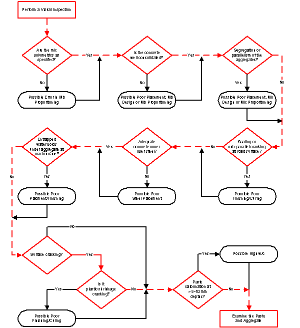
Figure 3-59. Flowchart for assessing general concrete properties based on visual examination as applied to NC-440-015.
|
Possible Distress |
Present |
Additional Information |
|
|---|---|---|---|
|
Shrinkage Cracks or Sample Preparation Cracks |
Yes |
No |
See Recommended Literature |
|
Paste Freeze-Thaw |
Yes |
No |
Table II-2 |
|
Aggregate Freeze-Thaw |
Yes |
No |
Table II-3 |
|
Sulfate Attack |
Yes |
No |
Table II-4 |
|
Deicer Attack |
Yes |
No |
Table II-5 |
| Secondary Deposits |
Yes |
No |
Figure 3-62 |
Figure 3-60. Flowchart for assessing the condition of the concrete paste as applied to NC-440-015.
|
Possible Distress |
Present |
Additional Information |
|
|---|---|---|---|
|
Natural Cracking of Aggregate |
Yes |
No |
See Recommended Literature |
|
Sample Preparation Cracks |
Yes |
No |
See Recommended Literature |
|
Aggregate Freeze Thaw |
Yes |
No |
Table II-3 |
|
Natural Weathering of Aggregates |
Yes |
No |
See Recommended Literature |
|
Alkali-Silica Reaction |
Yes |
No |
Table II-6 |
|
Alkali-Carbonate Reaction |
Yes |
No |
Table II-7 |
|
Secondary Deposits
|
Yes |
No |
Figure 3-62 |
Figure 3-61. Flowchart for assessing the condition of the concrete aggregates as applied to NC-440-015.
|
Possible Distress |
Present |
Additional Information |
|
|---|---|---|---|
|
Sulfate Attack |
Yes |
No |
Table II-4 |
|
Deicer Attack |
Yes |
No |
Table II-5 |
|
Alkali-Silica Reaction |
Yes |
No |
Table II-6 |
|
Alkali-Carbonate Reaction |
Yes |
No |
Table II-7 |
| Corrosion of Embedded Steel |
Yes |
No |
Table II-1 |
Figure 3-62. Flowchart for identifying infilling materials in cracks and voids as applied to NC-440-015.
Table 3-23. Diagnostic features identified along with their associated MRD type and significance as related to NC-440-015.
|
Diagnostic |
Method of Characterization |
Associated with MRD Type |
Significance |
|---|---|---|---|
|
Secondary deposits filling air voids and cracks |
Visual |
Paste freeze-thaw, Deicer attack, Sulfate attack (both internal and external) |
Low |
|
Inadequate air-void system |
Visual |
Paste freeze-thaw |
Low |
|
Microcracking around aggregates |
Stereo OM |
||
|
Map cracking without exudate |
ASR |
Medium |
|
|
ASR reaction products in cracks and voids |
Petrographic OM |
High |
|
|
Reaction rims on aggregates |
Petrographic OM |
Low |
|
|
Microcracking radiating from reacted aggregates |
Stereo OM |
Medium |
|
|
Significant sulfate deposits in cracks and voids |
Staining |
Sulfate
attack |
Low |
Using the procedures presented in Guideline III in Volume 2: Guidelines Description and Uses, feasible treatment and rehabilitation alternatives were selected. The most significant MRD mechanism found was ASR. The deterioration is characterized as map cracking (hairline) over the entire pavement surface, with some associated staining. Isolated areas of higher deterioration were noted, necessitating patching. The severity level would be classified as medium severity, with some isolated areas of high severity. As a result, feasible treatment/rehabilitation alternatives include:
Ultimately, as the pavement continues to deteriorate, a reconstruction/recycling option becomes more viable. If recycling is considered, precautions must be taken to avoid ASR in the newly constructed pavement.
For the distresses noted, the best preventative strategy is to use a source of aggregate that is not ASR susceptible. Testing in accordance with the guidelines should show that the current source would be unacceptable without mitigation. Mitigation strategies for ASR that could be used if the current aggregate source is all that is available include:
If aggregate benefaction is not feasible or cost effective, other strategies can be employed including:
Regardless of the approach, the design PCC mixture must be tested to ensure that the ASR has been mitigated.
This project is located on State Route 58 near Boron, California. This particular project has been documented in the literature as exhibiting cracking patterns typically associated with ASR (Stark et al. 1993). The project was constructed in 1970 and has exhibited MRD for many years. In 1988, the project was treated with HMWM. After an evaluation of several other possible projects located in California, this project was selected as the primary case study to represent the dry-nonfreeze climatic region. Los Angeles, which is the closest major metropolitan area, has an annual precipitation of about 300 mm and no degree-days below freezing.
State Route 58 is a four-lane divided highway running east and west. However, the test project is located in the eastbound lanes only, extending from milepost 141.8 to milepost 142.5. A summary of the design information for this project is presented in table 3-24. The pavement is a 230-mm JPCP with a variable (4.0-5.8-5.5-5.7 m) joint spacing. The transverse joints are skewed at a angle of 1-to-6 (longitudinal-to-transverse). No load transfer mechanisms are provided at the longitudinal or transverse joints. The inside and outside shoulders, both of which have an AC surface, are 1.2 and 3.0 m wide, respectively.
Chemistry lab data from the construction records indicated that the soil sulfate composition at this site was less than 200 ppm. As a result, this test site would be classified as a moderate sulfate exposure in accordance with ACI 201.2R-92.
Table 3-24. Summary of design features for CA-058-141.
|
Category |
Design Feature |
Description |
|---|---|---|
|
General |
Project limits |
MP 141.8 - 142.5 |
|
Highway type |
Divided |
|
|
Number of lanes |
4 |
|
|
Direction |
Eastbound |
|
|
Construction date |
1970 |
|
|
Cumulative ESALs |
||
|
Pavement |
Pavement type |
JPCP |
|
PCC slab thickness |
230 mm |
|
|
Base |
||
|
Subbase |
||
|
Subgrade type |
Sand |
|
|
Transverse |
Joint spacing |
4.0-5.8-5.5-3.7 m |
|
Joint skew |
1:6 |
|
|
Load transfer |
Aggregate interlock |
|
|
Sealant type |
None |
|
|
Longitudinal |
Load transfer |
Aggregate interlock |
|
Sealant type |
None |
|
|
Outer |
Surface type |
AC |
|
Width |
3.0 m |
|
|
Inner |
Surface type |
AC |
|
Width |
1.2 m |
|
|
Climatic |
Region |
Dry-nonfreeze |
|
Annual precipitation |
305 mm (in Los Angles) |
|
|
Freezing index |
0°C-days (in Los Angles) |
This project is a relatively short project that exhibits significant MRD throughout its entire length. The section selected for detailed investigation under this study begins at milepost 141.8 and extends 150 m to the east. This section was constructed on approximately 2.5 m of fill material. Table 3-25 presents a summary of the distress survey results for Section 001.
Map cracking is located throughout the entire pavement area. The only other noteworthy distresses are spalling and patching, both of which are due to deterioration of the surface cracking. Five of the 33 transverse joints have joint spalling over a portion of its length (4 have progressed to medium severity). There are seven small AC patches, all of which are medium severity, that have been placed to address the spalling caused by surface cracking. Even though the joints do not contain any load transfer devices, faulting is not significant enough to affect ride quality.
Table 3-25. Summary of pavement condition surveys for CA-058-141-001.
|
Distress Type |
Distress Measure |
Severity Level |
Comments |
|||
|---|---|---|---|---|---|---|
|
Low |
Moderate |
High |
||||
|
Cracking |
Corner Breaks |
number |
0 |
0 |
0 |
|
|
Longitudinal Cracking |
linear meters |
0.0 |
0.0 |
0.0 |
||
|
Transverse Cracking |
number of cracks |
0 |
0 |
0 |
||
|
linear meters |
0.0 |
0.0 |
0.0 |
|||
|
percent of slabs |
0 |
|||||
|
Transverse Joints |
Sealant |
n/a |
not sealed |
|||
|
Spalling |
number |
1 |
4 |
0 |
||
|
linear meters |
0.1 |
1.3 |
0.0 |
|||
|
Faulting |
millimeters |
1.3 |
measured at 0.30 m |
|||
|
millimeters |
0.6 |
measured at 0.75 m |
||||
|
Width |
millimeters |
3.4 |
||||
|
Long. Joints |
Sealant |
n/a |
not sealed |
|||
|
Spalling |
linear meters |
0.0 |
0.0 |
0.0 |
||
|
Shoulder Dropoff |
millimeters |
3.4 |
||||
|
Surface Conditions |
Map Cracking |
number of slabs |
32 |
all slabs affected |
||
|
square meters |
561.0 |
entire area |
||||
|
Scaling |
number of slabs |
0 |
||||
|
square meters |
0.0 |
|||||
|
Polished Aggregate |
square meters |
0.0 |
||||
|
Popouts |
number/sq. meter |
0.0 |
||||
|
Other |
Blowups |
number |
0 |
|||
|
Flexible Patches |
number |
0 |
7 |
0 |
||
|
square meters |
0.0 |
0.8 |
0.0 |
|||
|
Rigid Patches |
number |
0 |
0 |
0 |
||
|
square meters |
0.0 |
0.0 |
0.0 |
|||
|
Pumping/Bleeding |
number |
0 |
||||
|
linear meters |
0.0 |
|||||
During the distress surveys, detailed information was collected to characterize the MRD. This information is useful, in conjunction with a laboratory investigation, to help diagnose the type and cause of MRD. Table 3-26 summarizes the key attributes of the MRD.
Table 3-26. Summary of MRD characterization for CA-058-141.
|
Description |
Section 001 |
Comments |
|
|---|---|---|---|
|
Cracking |
Location |
Entire slab |
|
|
Orientation/shape |
Honeycomb |
||
|
Extent |
Entire slab |
||
|
Crack size |
Hairline/open |
Longitudinal cracks are more open; spalling at interconnecting cracks |
|
|
Staining |
Location |
Around cracks |
|
|
Color |
Dark gray |
||
|
Exudate |
Present |
Yes |
Not observed at all cracks |
|
Color |
White |
||
|
Extent |
Low |
||
|
Scaling |
Location |
None |
|
|
Area of surface |
n/a |
||
|
Depth |
n/a |
||
|
Vibrator Trails |
Visible |
None |
|
|
Discolored |
n/a |
||
|
Distressed |
n/a |
||
|
Change in texture |
n/a |
||
As described previously, the MRD on this project is characterized by map cracking over the entire pavement surface. The most predominant cracking at the surface runs parallel to the longitudinal joints. These cracks are more prevalent, wider, and more deteriorated than the cracks running in other directions. In more deteriorated areas, the transverse and diagonal surface cracks have interconnected, forming a criss-cross or honeycomb pattern. These interconnecting cracks have led to spalling and loose material on the pavement surface.
A dark gray staining has occurred in the area surrounding the cracks. However, due to the extensive cracking, the entire pavement surface has a darker appearance. The cracks were once sealed with an HMWM, but that material does not appear to be performing its intended function at this time. Although not widespread, exudate, typically white in color, is observed at a few cracks. Figure 3-63 shows typical distress patterns for this site.
Core Selection/Visual Inspection
Based upon the field survey, distress was widespread. The joints were badly deteriorated and coring at the transverse joint produced pieces rather than an intact core. Cores C, D, and E were relatively intact and were thus analyzed. Photos of these cores are shown in figure 3-64. All cores were cut to produce slabs for examination with stains.
Figure 3-63. Typical conditions at CA-058-141.
Figure 3-64. Photographs of core specimens analyzed from CA-058-141.
Mix proportions were estimated by inspecting the cores visually before and after slicing. In this case, construction records were unavailable to verify the mix design. The concrete was well consolidated with no apparent segregation or parallelism of the aggregates. No scaling or sub-parallel cracking was apparent on these sites. No entrapped water voids were seen under aggregates or embedded steel. Surface cracking was apparent that was not plastic shrinkage cracking. Darkened reaction rims were seen around some of the coarse aggregates. Abundant cracks filled with white deposits were visible with the unaided eye. The coarse aggregates used were a natural igneous (both intrusive and extrusive) and the natural fine aggregate used appear to be similar in lithology.
For this study, the stereo optical microscope was used primarily for observing stained specimens, selecting areas for preparing thin sections, and air void analysis. In this climate, air content is not an important factor in MRD unless it becomes excessive. Interestingly enough, according to the construction records obtained, this concrete was air entrained. As a result, only two cores were analyzed using ASTM C 457. A wide disparity in air content is noted but not considered abnormal considering the small sample size of only two cores. Also, a side benefit of performing the ASTM C 457 test is obtaining a measure of the relative phase abundance in the concrete. The results of the analysis are presented in table 3-27.
Table 3-27. Results of ASTM C 457 on concrete from CA-058-141.
|
Core |
Original |
Existing |
Volume Percent |
||||
|---|---|---|---|---|---|---|---|
|
Air Content |
Spacing Factor |
Air Content |
Spacing Factor |
Paste |
Coarse Aggregate |
Fine Aggregate |
|
|
Site 1 Core C |
1.9 |
0.230 |
1.1 |
0.430 |
23.0 |
54.3 |
20.9 |
|
Site 1 Core D |
5.7 |
0.305 |
5.7 |
0.338 |
27.2 |
44.9 |
22.2 |
Cores C and D were slabbed and stained using the sodium cobaltinitrite stain for identifying ASR reactive aggregates and reaction products. Also, slabs were stained with the potassium permanganate/barium chloride stain for identifying sulfate minerals. ASR reaction product was seen in cracks associated with the coarse aggregate. Ettringite was common in cracks and voids, and actually was more common than ASR reaction product. Examples of these stains as applied are shown in figure 3-65.
|
|
|
|
(a) Sodium cobaltinitrite yellow stain picked up in crack within felsic volcanic coarse aggregate |
(b) An unpolished cut surface that has been stained to show ettringite filled cracks and voids |
Figure 3-65. Stereo optical micrographs showing staining observed in core CA-058-141-001C.
Petrographic Optical Microscopy
Petrographic microscopy confirmed what was seen visually and by stereo optical microscopy. Alkali-silica gel was present in some cracks associated with some coarse aggregate, primarily felsic volcanics. Ettringite was common in cracks and air voids. This is seen in figures 3-66 and 3-67.
In this case, the SEM was used simply as a means of confirming the results of the petrographic optical microscopy, stereo optical microscopy, and visual inspection. Using x-ray microanalysis, the ASR gel deposits shown in figure 3-68 were analyzed and these results are summarized in table 3-28. Many ettringite filled cracks were observed and an example is shown in the back-scattered electron (BSE) micrograph shown in figure 3-68.
|
|
|
|
(a) Typical spectrum from ASR gel adjacent to volcanic aggregate pictured in (b). |
(b) BSE image of ettringite filling a crack along the contact between a coarse aggregate and the cement paste. |
Figure 3-68. SEM spectra and micrograph from CA-058-141.
Table 3-28. Summary of 12 analyses of ASR gel deposit shown in figure 3-68.
|
Element |
Average Wt% |
Standard Deviation % |
|---|---|---|
|
Na |
0.5 |
0.3 |
|
Mg |
0.6 |
2.3 |
|
Al |
0.2 |
0.5 |
|
Si |
20.4 |
1.6 |
|
S |
0.0 |
0.0 |
|
Cl |
0.0 |
0.1 |
|
K |
0.8 |
0.6 |
|
Ca |
28.8 |
6.0 |
|
Ti |
0.0 |
0.0 |
|
Mn |
0.0 |
0.0 |
|
Fe |
0.0 |
0.1 |
|
O |
Not Measured |
|
|
H |
Not Measured |
|
|
sum |
51.2 |
|
Having performed the described laboratory analyses and applied the diagnostic flow charts, shown in figures 3-69 through 3-73, two possible MRDs were identified in CA-058-141, including sulfate attack and ASR, with ASR being the dominant MRD. To finalize the diagnosis, the diagnostic tables were consulted. In this case, the diagnostic tables were being used as a review to ensure that no possible MRD was overlooked. The diagnostic features identified in the analysis processes are listed below in table 3-29 along with their associated MRD type and significance as related to this pavement. A brief discussion of each distress is given below:
ASR - In consulting the diagnostic tables, the only other possibility other than ASR is some form of sulfate attack. However, according to the construction records, Type II modified cement was specified, which should provide protection from the moderate sulfate exposure. As a result, ASR is the most likely cause. The reaction was extensive and clearly documented in the laboratory analysis.
External Sulfate Attack - The large amounts of ettringite present are significant but may be opportunistic. Given the fact that Type II cement was used and there was no evidence of ettringite formation within the paste, sulfate attack is ruled out. In general, without clear evidence of ettringite forming within the hardened paste, sulfate attack is unlikely.
Although many would argue that guidelines are not needed on such an "obvious" distress, the guidelines are useful because the analyst is not allowed to make a final judgment until all the data are in. In this case, construction records provided the final piece of data (i.e., the soil sulfate content) and without pulling all sources of data together, clues about other possible distresses may be missed.
Using the procedures presented in Guideline III in Volume 2: Guidelines Description and Uses, feasible treatment and rehabilitation alternatives were selected. The two most significant MRD mechanisms found were ASR and external sulfate attack. Because the two mechanisms are acting in concert, it is difficult to rate the severity of each independently. The distress is characterized by high severity map cracking over the entire pavement surface accompanied by exudates, spalling, and patching. The severity level would thus be assigned as high severity whether it is ASR or sulfate attack. As a result, feasible treatment/rehabilitation alternatives include:
If recycling is considered, precautions must be taken to avoid ASR and/or sulfate attack in the newly constructed pavement.
Figure 3-69. Flowchart for assessing the likelihood of MRD causing the observed distress in the pavement as applied to CA-058-141.
|
Possible Distress |
Present |
Additional Information |
|
|---|---|---|---|
|
Error in Mix Proportioning |
Yes |
No |
See Recommended Literature |
|
Poor Placement |
Yes |
No |
See Recommended Literature |
|
Poor Finishing/Curing |
Yes |
No |
See Recommended Literature |
|
Poor Steel Placement |
Yes |
No |
See Recommended Literature |
|
Carbonation at Depths > 5-10 mm |
Yes |
No |
See Recommended Literature |
Figure 3-70. Flowchart for assessing general concrete properties based on visual examination as applied to CA-058-141.
|
Possible Distress |
Present |
Additional Information |
|
|---|---|---|---|
|
Shrinkage Cracks or Sample Preparation Cracks |
Yes |
No |
See Recommended Literature |
|
Paste Freeze-Thaw |
Yes |
No |
Table II-2 |
|
Aggregate Freeze-Thaw |
Yes |
No |
Table II-3 |
|
Sulfate Attack |
Yes |
No |
Table II-4 |
|
Deicer Attack |
Yes |
No |
Table II-5 |
|
Secondary Deposits |
Yes |
No |
Figure 3-73 |
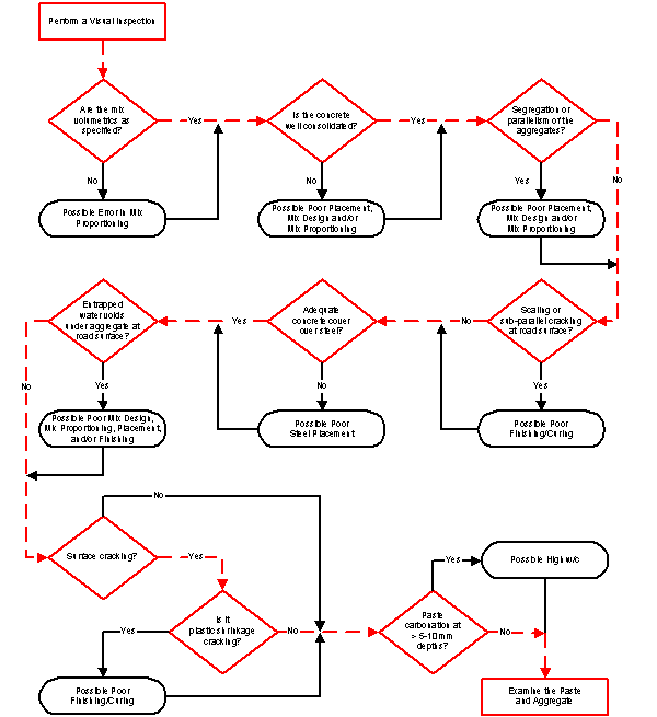
Figure 3-71. Flowchart for assessing the condition of the concrete paste as applied toCA-058-141
|
Possible Distress |
Present |
Additional Information |
|
|---|---|---|---|
|
Natural Cracking of Aggregate |
Yes |
No |
See Recommended Literature |
|
Sample Preparation Cracks |
Yes |
No |
See Recommended Literature |
|
Aggregate Freeze Thaw |
Yes |
No |
Table II-3 |
|
Natural Weathering of Aggregates |
Yes |
No |
See Recommended Literature |
|
Alkali-Silica Reaction |
Yes |
No |
Table II-6 |
|
Alkali-Carbonate Reaction |
Yes |
No |
Table II-7 |
|
Secondary Deposits
|
Yes |
No |
Figure 3-73 |
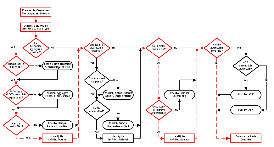
Figure 3-72. Flowchart for assessing the condition of the concrete aggregates as applied to CA-058-141.
|
Possible Distress |
Present |
Additional Information |
|
|---|---|---|---|
|
Sulfate Attack |
Yes |
No |
Table II-4 |
|
Deicer Attack |
Yes |
No |
Table II-5 |
|
Alkali-Silica Reaction |
Yes |
No |
Table II-6 |
|
Alkali-Carbonate Reaction |
Yes |
No |
Table II-7 |
| Corrosion of Embedded Steel |
Yes |
No |
Table II-1 |
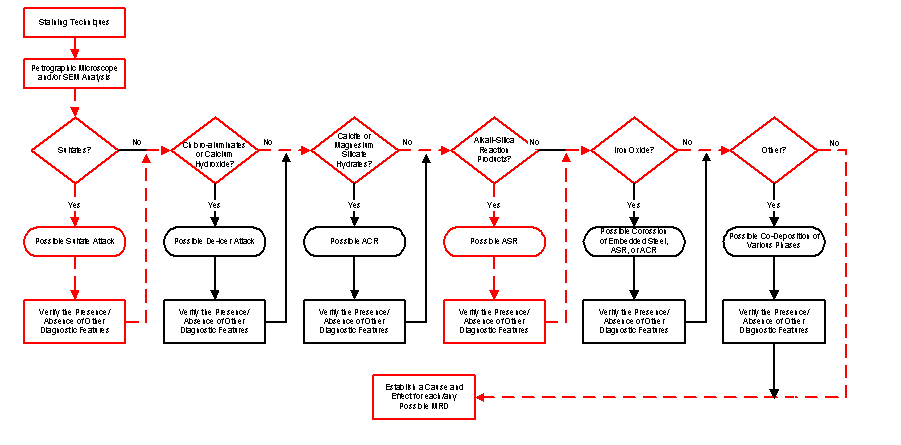
Figure 3-73. Flowchart for identifying infilling materials in cracks and voids as applied to CA-058-141.
Table 3-29. Diagnostic features identified along with their associated MRD type and significance as related to this pavement.
|
Diagnostic |
Method of Characterization |
Associated with MRD Type |
Significance |
|---|---|---|---|
|
Map cracking without exudate |
ASR |
Medium |
|
|
ASR reaction products in cracks and voids |
Petrographic OM |
High |
|
|
Reaction rims on aggregates |
Petrographic OM |
Low |
|
|
Microcracking radiating from reacted aggregates |
Stereo OM |
Medium |
|
|
Significant sulfate deposits in cracks and voids |
Staining |
Sulfate attack |
Low |
|
External source |
Construction records |
External sulfate attack |
Medium |
For the distresses noted, the best preventative strategy is to use a source of aggregate that is not ASR susceptible and a cement type and w/c combination that will not deteriorate under moderate sulfate conditions. Testing in accordance with the guidelines should show that the current aggregate source would be unacceptable without mitigation. Mitigation strategies for ASR include aggregate benefaction using the following strategies:
If aggregate benefaction is not feasible or cost effective, other strategies can also be employed including:
Sulfate attack is typically mitigated by using a different cement (such as Type II or V), adding supplementary cementitious materials such as a pozzolan or ground slag, and/or reducing the w/c. For moderate sulfate conditions, Type II, IP(MS), or IS(MS) cement should be used, or a blend of Type I cement and a GGBFS or a pozzolan that has been determined by tests to give equivalent sulfate resistance. Further, a maximum w/c of 0.5 is recommended.