Chapter 3. Results and Discussion

Currently, this study has involved a number of specimens to obtain the following results. ECE studies have been completed on 20 of the Type I and 12 of the Type II test blocks. These blocks included different cover depths, which ranged from 3.5 cm to 6.4 cm. To evaluate the affect of the w/c ratio on ECE, test blocks with ratios ranging from 0.40 to 0.60 were designed. Descriptions of the block designs are presented in tables 7 through 12 and illustrated in figures 4 and 5.

Changes in the Current and Voltage during ECE

During ECE, the current was monitored, while internal and external voltage measurements were made. The designations in the following graphs to the different measurement points that were monitored during ECE for the Type I and Type II test blocks are listed in tables 11 and 12, respectively. Figures 4 and 5 can provide additional insight into the connections used to make measurements.

The typical change in voltage during ECE for a set of Type I specimens with different w/c ratios, but the same cover depth is shown in figure 10. The benefit of these specimens was the ability to measure the voltage changes in different layers between the anode and cathode. Under constant voltage conditions, it can be seen that the voltage between the anode and the upper titanium rods increases. At the same time, the voltage between the lower titanium rods and the reinforcing steel is decreasing. In each case, the rate of change of the voltage is greatest initially, i.e., during the first 10 to 15 days, and then the rate of change decreases for the remaining extraction period. All of the specimens evaluated exhibited this type of behavior. Even with larger applied voltages, the voltage difference in the top layer of concrete increased during ECE. A typical example of this is shown for two specimens in figure 11. As the applied voltage to the slab increases under constant current conditions, the voltage across the top layer of concrete increases.

Figure 10. Measured voltage changes during ECE in a set of Type I specimens (Maximum voltage was 9V)

Figure 11. Comparison of the voltages measured between (1) the anode and rebar and
(2) between the anolyte and the titanium strip in the concrete. Top: for a 0.55-w/c Type II
specimen; Bottom: for a 0.50-w/c Type II specimen (Maximum voltage was 40V)

Influence of Concrete Surface on Voltage and Current

To better understand the influence of the surface-layer concrete on the voltage and current, one of the Type I specimens was subjected to an extended ECE experiment and analysis. A timeline illustrating the sequence of events that took place in this extended experiment is shown in figure 12. First, the specimen was ECE treated or polarized for 26 days and then depolarized for 38 days. The voltage and current data for this 26-day ECE treatment are shown in figure 13a. Then, the specimen was re-energized for 12 hours. The voltage and current data for this first 12-hr polarization are shown in figure 13b. This was followed by removal and storage of the electrolyte used during the ECE test period. The surface of the concrete was then sandblasted and the stored electrolyte was poured back into the reservoir. After allowing twenty hours for the solution to soak into the concrete, ECE was initiated again for another 12 hours and the same measurements were made (figure 13c). Finally, the sample was depolarize for 36 hours and then re-energized for a final 12-hour duration and a final set of measurements was made (figure 13d).

Comparison of figures 13a and 13b would indicate that the voltages and current of the system at the start of the first 12-hour re-polarization were practically the same as where the system was at the end of the 26-day of polarization. Comparison of figures 13b and 13c would reveal the effect of the sandblasting the surface layer concrete on the voltages and current. It is clear that sandblasting the surface of this specimen increased the current density by over 0.3 A/m². This current density was even greater than the initial current density value (at the beginning of the 26-day treatment). Following sandblasting, the voltage between the anode and the reinforcing steel also switched from constant-voltage mode to constant-current mode, but then returned to a constant-voltage mode. In addition, sandblasting resulted in voltage changes within the different concrete regions, which are on the order of approximately 2 V. This indicates that the surface of the concrete appears to have a significant influence on the voltage and current during ECE. However, additional testing on other specimens will be required to confirm these observations.

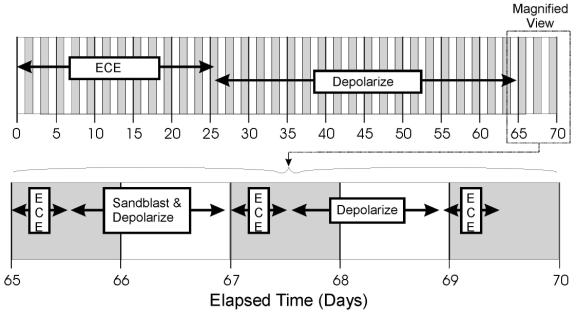
Figure 12. Timeline of concrete surface study

Figure 13. Influence of concrete exterior surface on the voltage and current in a 0.45-w/c Type I specimen

Changes in the Concrete Resistance During ECE

The resistance between different points in the concrete was determined using the IR Drop technique, which was discussed in the earlier section "IR Drop Measurements" on page sixteen. During ECE, the resistance was observed to increase in the region between the anode and the upper layer of titanium rods, as shown in figure 14. In contrast, the solution (concrete) resistance decreased in all other regions during ECE. A comparison, based on w/c ratios, of the resistance between the anode and the upper titanium rods did not indicate an obvious relationship. This pattern was consistent in all of the samples studied.

Figure 14. Example showing the change in resistances for a single set of Type I specimens during ECE

Resistivity

It was apparent that, immediately before ECE, the resistivity of the top layer of concrete, as measured by the upper row of four titanium rods, was less than that of the lower concrete that surrounded the lower set of four titanium rods, as shown in figure 15. This difference was observed in the other specimens prior to ECE. It is also apparent in figure 15 that the resistivity of the lower region of the concrete undergoes only a relatively slight to moderate change during ECE. In contrast, the resistivity of the top layer of concrete increased and exceeded that of the lower concrete and then remained at a level that is greater than that of the lower concrete region. However, a clear relationship between w/c ratio and resistivity for either the upper or lower titanium rod region was not evident. This is shown in figures 16 and 17, respectively.

Figure 15. Change in Resistivity for Type I specimens of various w/c ratios (cover thickness of 4.4 cm)

Figure 16. Resistivity change in the upper layer of concrete, for Type I Specimens with various w/c ratios (cover thickness of 4.4 cm)

Figure 17. Resistivity change in the lower layer of concrete, for Type I Specimens with various w/c ratios (cover thickness of 4.4 cm)

Chloride Concentration in Concrete with ECE

The previous data have shown that the concrete specimens studied behaved in a stratified manner during ECE. Generally, the resistivity in the upper layers of concrete increased while that at the lower layers decreased. Upon determining the chloride concentration before and after ECE in Type I specimens, it is evident that a large change in chloride concentration occurs near the surface adjacent to the anode, which is shown in figures 18 and 19. (The negative values in figures 18 and 19 indicate a decrease in chloride concentration; conversely, positive values signify an increase in chloride concentration.) It is apparent that significant removal of chlorides during ECE are occurring in the concrete layer near the anode. In contrast, the treated Type II specimens exhibited a more even removal distribution at deeper depths in the concrete, which is shown in figures 20 and 21.

Unlike the Type II specimens, the Type I specimens exhibited a decrease in chloride removal at deeper depths within the concrete and some specimens even display an increase in chloride concentration near the reinforcing steel. This is attributed to two factors: (1) the use of admixed chlorides in the Type I specimens and (2) the difference in the steel surface area in the different specimen types (table 13). It is possible that the admixed chlorides below the bar were drawn upward during ECE. In addition, these results support earlier studies that indicate the importance of available cathode area. The decreased cathode surface area in the Type I specimens appears to decrease the total current flow, which decreased the percentage of chloride removed. In the Type I specimens, 0% - 52% of the chlorides were removed during treatment, whereas 33% - 76% of the chlorides were removed from the Type II specimens.

Cover thickness appears to influence the quantity of chloride removed. However, additional samples must be evaluated to provide statistical validity to the observed trend.

Figure 18. Average change in chloride concentrations due to ECE in Type I specimens with
4.4 cm of concrete cover over rebar

Figure 19. Average change in chloride concentrations due to ECE in Type I specimens with
5.7 cm of concrete cover over rebar

Figure 20. Change in chloride concentrations due to ECE in a single set of Type II specimens
with 3.8 cm of concrete cover over rebar

Figure 21. Average change in chloride concentrations due to ECE in Type II specimens
with 6.4 cm of concrete cover over rebar

Visual Observations

After completing ECE, each specimen's surface was examined for physical changes. In each case, a tightly adhering substance had formed on the surface. Images of this formation are shown in figure 22. Attempts to remove the unknown material from the surface proved difficult. Upon trying to cleave it, a portion of the concrete was dislodging in addition to the unknown material. This provided a cross section of the interface, which is shown in figure 23. A surface formation following treatment has been found on actual treated bridge decks.^[70] As shown in figure 24, the formation parallels the reinforcing steel mat below. It is evident from these photographs that the surface formation creates perpendicular lines that crisscross the older concrete, as well as the recently repaired concrete (areas covered with more white material than their surrounding). Surface formation samples were collected and are currently being analyzed.

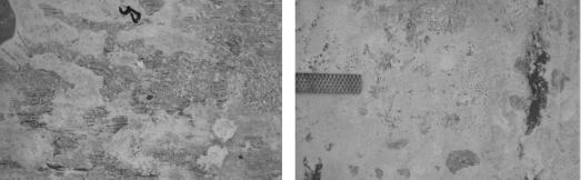
Figure 22. Tightly adhering layer of white material formed on the concrete surface during ECE

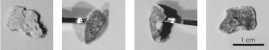
Figure 23. Various views of surface layer that formed on the concrete during
ECE: (Left) top view, (Middle) edge views, (Right) bottom view

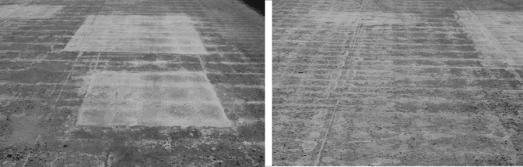
Figure 24. Layer of white material formed on the concrete surface directly
above the reinforcing steel following ECE on an actual bridge deck ^[70]

The increased current flow because of sandblasting the concrete surface, which removed the residue, was discussed earlier. That particular specimen is shown in figure 25. It is interesting to note that white deposits formed in the exposed pores, which is shown in the bottom photograph in figure 25. As indicated earlier, the study of new samples (shown in figure 27) will add statistical validity to the observed improvement in current flow following sandblasting. It is expected that removal of the tightly adherent surface formation will improve the ECE process.

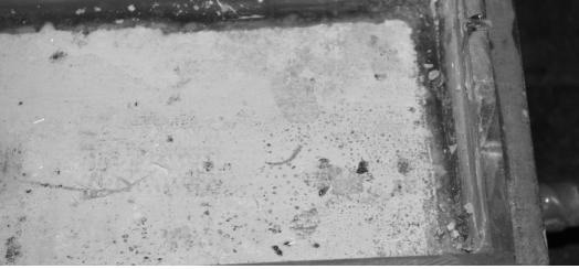
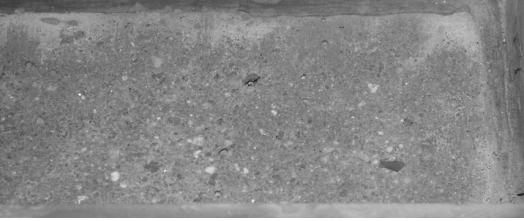
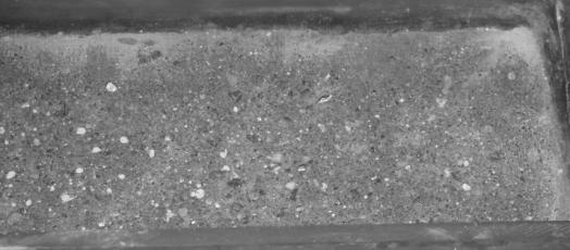
Figure 25. Type I specimen surface appearance: (Top) after ECE but prior to
sandblasting, (Middle) after sandblasting but prior to second application of
ECE, (Bottom) following a second application of ECE for 12 hours

Surface Deposit Analysis

To identify the white material covering the concrete surface following ECE, which is shown in figures 22 and 23, XRD was performed on two different Type II specimens. Calcium carbonate was clearly identified by XRD to be present in both specimens. Figure 26 is an overlay of a calcium carbonate spectrum over the top of the spectrum for one of the unknown samples. It is apparent that all of the peaks locations in the standard match the peaks locations in the unknown sample. However, the intensities differed, which indicates additional crystalline materials are most likely present in minute amounts in the sample. In addition, not all of the peaks in the unknown sample diffraction pattern are accounted for by the calcium carbonate standard. Based on these observations, calcium carbonate appeared to be the major component in the white residue; however, the presence of other components in trace quantities is evident. The XRD spectrum from the other sample analyzed displayed the same characteristics as those found in the sample shown in figure 26. Table 15 lists the intensities and peak positions for the two samples examined.

XPS was also performed on the white material deposited on one Type I specimen and one Type II specimen. The Type I specimen used calcium hydroxide as the electrolyte, whereas industrial lime was used as the electrolyte for the Type II specimen. The XPS data indicated that calcium chloride was present on the surface of both samples. In addition, XPS detected magnesium in the sample exposed to a solution of industrial lime, but magnesium was not present in the sample that used reagent grade calcium hydroxide as the electrolyte. Work is underway to evaluate the significance of these finding through ongoing analysis on additional samples. Table 16 lists the elements and binding energies for the two samples examined.

Figure 26. Surface deposit XRD pattern from a Type II specimen comparing the
unknown material to calcium carbonate

Table 15. Surface deposit peak data using x-ray diffraction

Table 16. Surface deposit peak data using x-ray photoelectron spectroscopy