Chapter 2. Experimental Method

Two types of reinforced concrete specimen designs are being used during this portion of the study. Tables 7 and 8 list the basic design features of each type of specimens. These specimens included variations in the method of introducing chlorides into the concrete, cover thickness, and w/c ratios. Tables 9 and 10 list the mix designs for the Type I and II concrete specimens, respectively. After the specimens had cured, a dam was affixed to the top of each specimen to hold the appropriate solutions. The Types I blocks were kept in a controlled laboratory environment, whereas Type II blocks were exposed outside to further simulate field conditions.

As illustrated in figure 4, the Type I specimens were designed with two rows of activated titanium rods embedded in the concrete above the reinforcing steel bar. Each row has four activated titanium rods aligned in a horizontal plane at 1.0 cm below the top concrete surface and 1.0 cm above the rebar. This arrangement allowed for the measurements of the IR drop and voltage differences at selected depths during an ECE experiment. A list of these points is provided in table 11. In addition, these rows of embedded titanium electrodes allowed for measurement of the changes in the concrete resistivity at the two depths, using the four-pin method (ASTM G-57).

Each Type II concrete specimen contained a thermocouple, two titanium-mesh ribbon strips, and a corrosion probe embedded in the concrete, as illustrated in figure 5. The thermocouple was located 3.8 cm from the surface and horizontally centered in the sample. Each titanium mesh ribbon was 1.3 cm wide and 5.1 cm long. The two ribbons were 6.35 cm apart and located 1.0 cm below the surface. The corrosion probe was a graphite reference electrode and a 1.3-cm wide titanium counter electrode, all encased in concrete. Before casting the specimens, the probe was attached to the upper reinforcing steel mat. Table 12 lists the various contact points between which measurements can be made during ECE experiments on these specimens.

Table 13 lists the differences in some of the physical characteristics of Type I and II concrete specimens being used in this study.

Table 7. Description of Type I concrete test blocks

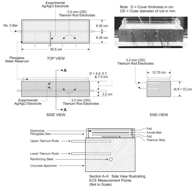
Figure 4. Illustration of a Type I Specimen

Table 11. Description of contact points used to make measurements in Type I concrete test blocks

* Based on the interior dam dimensions (9.5 cm X 26.1 cm)
** Based on the interior dam dimensions (60.96 cm X 60.96 cm)

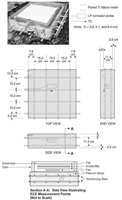
Figure 5. Illustration of a Type II Specimen

Electrochemical Chloride Extraction

Chlorides were extracted from the concrete specimens following the methods employed in previous ECE projects. The ECE parameters used are listed in table 14. In each experiment, a titanium-mesh anode and two pieces of felt were cut to fit the inside dimensions of the dam. A piece of felt was placed on the surface of the concrete inside the dam, which was followed by the titanium-mesh anode, and finally the titanium mesh was covered by a second piece of felt. The sandwiching of the titanium mesh between the felt ensured the complete wetting of the titanium-mesh anode. The anolyte was carefully added until the solution level inside the dam completely covered the upper felt mat. Either a saturated calcium hydroxide solution or a lime and water solution were used as the anolyte during ECE. A DC power supply was set to operate in constant current mode (1 A/m²) until it reached the maximum voltage output, at which time it would switch from constant current to constant voltage mode. The maximum voltage setting was dependent on the power supply. For the Type II specimens the maximum voltage was 40 V. A maximum of 40 V was also applied to one Type I specimen from each of the four w/c ratios studied, all of which had a cover thickness of 1.7 cm. For all other Type I specimens, the maximum voltage was between 9 V and 15 V. The positive lead from the power supply was attached to the anode and the negative lead to the reinforcing steel mat. To minimize the evolution of chlorine during ECE, the pH was maintained above 10 by adding either calcium hydroxide or lime to the anolyte.

Table 14. ECE parameters

Current and Voltage Measurements

Current and voltage measurements were made using a Tetronix digital multimeter or an IO Tech Logbook data acquisition system. With both instruments, voltage measurements were made directly. The current was calculated using the measured voltage across a resistor of known resistance and Ohm's law.

IR Drop Measurements

The total electrochemical cell voltage is the sum of a series of contributions from individual voltage differences.^[63] In simplest terms, these contributions are comprised of a thermodynamic potential difference (E_thermo), anodic and cathodic overpotentials (h_a and h_c, respectively), and the voltage drop due to current flow through a resistive solution (IR_sol).^[63-65] During ECE, the measured voltage difference (E_meas) is represented by equation 9 since the system is being driven.^{[64, 65]} Figure 6 illustrates this relationship graphically.

(9)

If the applied current is rapidly interrupted and the change in voltage is quickly recorded, the IR_sol component of the total voltage can be determined, as shown in figure 7.^[66] In the galvanostatic case, the solution resistance, R_sol, can be easily determined by dividing the measured voltage drop with the current.

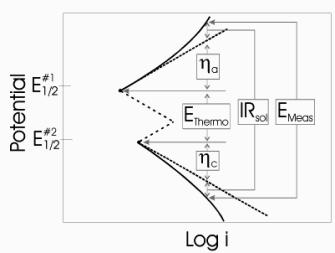
Figure 6. Illustration of voltage components for a driven system ^[64]

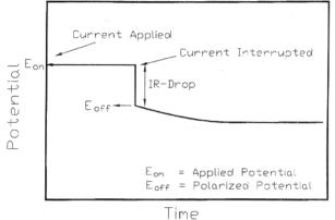
Figure 7. Change in voltage after interruption of applied current ^[66]

As with any measurement, care must be taken to minimize errors since this could yield misleading results. Therefore, the data acquisition system used must be capable of capturing events that are as short as a few milliseconds.^[66] Thompson and Payer suggested the use of an oscilloscope to capture IR-drop events.^[66] Moreover, since the current value is required to calculate the solution resistance, fluctuations in the current can significantly impair calculations of the solution resistance.^[66]

To guarantee the current interruption were reproducible, a solid-state relay controlled by a timing circuit was used to interrupt the current. Testing confirmed the solid-state relay interrupted the current in less than 6 ns. The timing circuit then maintained the solid-state relay in an open position for 13 ms.

To gather the voltage vs. time data, the IO Tech Logbook data acquisition system was used. To ensure the Logbook system would suffice, a HP 150MHz oscilloscope was used to verify that the Logbook acquisition rates were adequate. This was performed on circuits with known resistance values as well as on concrete test specimens. Following a series of successful comparisons between the two instruments, evaluations of Type I specimens began using the Logbook system. The Logbook acquisition system was set to gather data during periodic interruptions of the ECE process. Although the total current interruptions lasted for only 13 ms, data was gathered before, during, and after the interruption. This data was then used to determine changes in the IR-drop during ECE.

4-Pin Resistivity Measurements

As discussed earlier, the Type I concrete specimens were designed with the intention of making resistivity measurements during ECE. This was performed following ASTM Standard G 57, and using a Nilsson Soil Resistance Meter, Model 400. ^[67] This type of meter induces an AC signal between two outer pins while the voltage drop is measured between two inner pin, which is illustrated in figure 8.^[67] The output from this meter is in units of ohms (resistance), and therefore if the pins are evenly spaced and the inner pin spacing (a) is known, the resistivity (r) can be calculated using the following equation.^{[67, 68]}

(10)

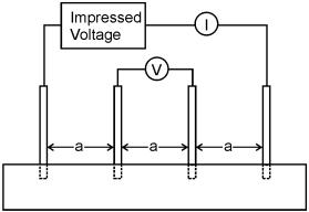
Figure 8. Four pin resistivity test method

Half-Cell Measurements

Half-cell measurements were made following the guidelines set forth in ASTM Standard C 876.^[69] Since these measurements were made on concrete surfaces, a damp sponge was used to ensure adequate contact between the half-cell and the concrete surface. Connectors were welded to each reinforcing steel mat, so that each piece of rebar was externally connected to each other. This ensured that the entire mat was conductive. In all cases, saturated Cu/CuSO₄ electrodes (CSE) were used to make measurements against the internal reinforcing steel mat.

Collection of Concrete Samples

To monitor the changes in chloride concentrations in the specimens during ECE, ground concrete samples were collected for chloride analysis from the specimens at different stages of the experiments, in accordance with AASHTO T 260. A sample collection scheme was used on the Type II specimens to minimize any possible interference that the collection of samples during the ECE experiment would impose on the current flow and voltage distribution in the specimen following the collection of concrete samples. Under this scheme, concrete samples were collected by starting on the outer perimeter of a specimen and working inward. An example of the sampling patterns used is shown in figure 9. At each time, three different points were sampled. For the blocks with a cover thickness of 6.4 cm, sampling was performed above a single bar. For the blocks with a cover thickness of 3.8 cm, sampling included the intersection of two bars, above a single bar, and where no bars were present. However, the same approach was not possible for the Type I specimen due to size constraints. In this case, the same technique for sample collection was used, but fewer samples were collected. Samples were collected before and after ECE in all cases. The sample depths were from the surface to 0.6 cm, 0.6 cm to 1.9 cm, 1.9 cm to 3.2 cm, and 3.2 cm to 4.1 cm. All of these depths were above the top reinforcing steel mat.

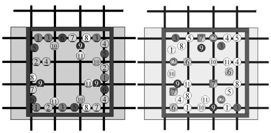
Figure 9. Type II specimen drill pattern for sample collection: Right, for a
cover thickness of 6.4 cm; Left, for a cover thickness of 3.8 cm

Potentiometric Titration

The acid-soluble chloride concentrations of the collected ground concrete samples were determined following AASHTO T 260. The analysis followed Method II in this standard, which uses the Gran Plot Method to determine the endpoint of the titration. A silver-ion-selective electrode was use during the titration.

X-Ray Diffraction

Surface residue that formed during ECE was analyzed using x-ray diffraction (XRD). It was anticipated that XRD would help in identifying any crystalline material in the residue. To accomplish this, residue samples were scraped from the surface and ground into a fine powder for analysis. These samples were then placed into the instrument for analysis.

XRD was performed using a Scintag automated diffraction system. During analysis, the applied voltage was 40 KV and the current was 35 mA. A copper target was used for the Kα x-ray source with a nickel filter to reduce undesirable components in the spectrum. The divergence and scatter slits on the source were 2 and 3, respectively. On the detector, the scattering and receiving slits were 1 and 0.5, respectively.

The XRD spectrum was evaluated using the program Diffraction Management System Software, version 1.1. Background subtraction was performed using a boxcar curve fit with a filter width of 1.5 degrees. The program's peak library software was used to compare the unknown sample against known spectra.

X-Ray Photoelectron Spectroscopy

To aid in identifying the composition of the residue that formed during ECE, a Perkin Elmer 560 system adapted for x-ray photoelectron spectroscopy (XPS) was used to analyze powder samples. Unlike XRD, which yields information about the bulk material in a sample, XPS provides surface information. The XPS data would be used to provide additional insight into the elements and compounds on the surface of the residue.

Charging effects during XPS analysis were adjusted for by setting the adventitious carbon line to 284.8 eV. Preliminary peak comparisons were first made against values cited in the literature. After reducing the possibilities, final identification was made against a sample of reagent grade calcium chloride.