U.S. Department of Transportation
Federal Highway Administration
1200 New Jersey Avenue, SE
Washington, DC 20590
202-366-4000


Skip to content
Facebook iconYouTube iconTwitter iconFlickr iconLinkedInInstagram

Federal Highway Administration Research and Technology
Coordinating, Developing, and Delivering Highway Transportation Innovations

Report
This report is an archived publication and may contain dated technical, contact, and link information
Publication Number: FHWA-HRT-04-124
Date: April 2005

Lab & Field Testing of AUT Systems for Steel Highway Bridges

6. RESULTS

Laboratory evaluation and field testing of the P-scan system in parallel with both RT and manual UT was performed on 10 laboratory specimens and 46 field specimens. The results produced from this testing illustrate the potential benefits of implementing AUT.

LABORATORY RESULTS TC "LABORATORY RESULTS"

The results of the laboratory evaluation are summarized in table 6. The first column of table 6 indicates the specimen identification code. The second, third, and fourth columns indicate the inspection method performed on each specimen. "Rejected" or "Accepted" indicates that the specimen was either rejected or accepted, respectively, by the employed inspection method. "Ind." stands for indication, and the angle (q) indicates the transducer's refracted angle. The indication characteristics in the fourth column (i.e., indication rating (d), length (L), depth (Z), x-position, and y-position) are obtained from P-scan images. These characteristics are compared with the UT acceptance-rejection criteria in tables 6.3 and 6.4 from the AASHTO/AWS D1.5M/D1.5: 2002 Bridge Welding Code(1) to determine whether the indication should be accepted or rejected.

The category 1 laboratory specimens were rejected by all three inspection methods (table 6). Figure 10 shows the radiographic image of laboratory specimen S033. Figure 12 shows the P-scan images of the toe and root cracks in specimen S033. The radiographic image provides the spatial dimensions of the defects (i.e., length and position), while the P-scan images provide three-dimensional information (including length, depth, and global position). Specimen S034 (figure 33) contained two manufactured cracks. This 12.7-mm- (0.5-inch-) thick plate contains a longitudinal crack in the weld (figure 34) and a transverse crack in the weld (figure 35). Both cracks were detected by RT and manual UT. Figure 36 shows the radiographic image of specimen S034. The two cracks can be seen clearly. The transverse crack in specimen S034 was detected by manual UT when the weld was inspected in the transverse direction. The P-scan system detected only the longitudinal/centerline crack in specimen S034 (figures 37 and 38). The photographs, radiographic images, and P-scan images of the remaining laboratory specimens that contained rejectable defects are shown in figures 39 through 71.

The results provided in table 6 showed that the indication rating (d) given by the P-scan system varied from the conventional UT rating in some cases. This variance may be caused by one of the following parameters:

  • High sensitivity of P-scan system.
  • Manual versus computer determination of spatial characteristics of defects (including sound path and time of flight).
  • Attenuation.
  • Slightly varying scanning patterns.
  • Operator variability.

Table 6. Inspection results of laboratory specimens.

Specimen ID

RT

Manual UT

AUT

S033

Rejected
Ind. 1: Toe Crack
Ind. 2: Root Crack

Rejected
Ind. 1: Toe Crack
Ind. 2: Root Crack


Rejected
Ind.1: Toe Crack
d = -3 dB
L = 2.45", Z = 0"
X = +0.13", Y = 0.57"
Ind. 2: Root Crack
d = -4 dB
L = 1.03", Z = 0.44"
X = -0.19", Y = 8.39"

S034

Rejected
Ind. 1: Centerline Crack
Ind. 2: Transverse Crack

Rejected
Ind. 1: Centerline Crack
Ind. 2: Transverse Crack

Rejected*
Ind. 1: Centerline Crack
d = 0 dB
L = 1.37", Z = 0.02"
X = +0.07", Y = 3.94"

*AUT is not configured to detect transverse cracks.
1 inch = 25.4 mm


Table 6. Inspection results of laboratory specimens (continued).

Specimen ID

RT

Manual UT

AUT

S125

Rejected


Rejected
Ind. 1: theta symbol = 70°
d = -1 dB
L = 0.38", Z = 0.63"
X = -0.38", Y = 2.25"
Ind. 2: theta symbol = 70°
d = +6 dB
L = 0.50", Z = 0.50"
X = 0", Y = 7.50"
Ind. 3: theta symbol = 70°
d = +7 dB
L = 0.25", Z = 0.33"
X = 0", Y = 13.38"

Rejected
Ind. 1: theta symbol = 70°
d = +3 dB
L = 0.55", Z = 0.65"
X = -0.34", Y = 2.29"
Ind. 2: theta symbol = 70°
d = +6 dB
L = 0.47", Z = 0.35"
X = +0.053", Y = 7.81"
Ind. 3: theta symbol = 70°
d = +8 dB
L = 0.23", Z = 0.39"
X = +0.09", Y = 13.32"

S126

Rejected

Rejected
Ind. 1: theta symbol = 70°
d = -2 dB
L = 1.25", Z = 0.82"
X = -0.25", Y = 2.5"
Ind. 2: theta symbol = 70°
d = +5 dB
L = 0.63", Z = 0.69"
X = +0.25", Y = 6.88"
Ind. 3: theta symbol = 70°
d = +11 dB
L = 0.50", Z = 0.25"
X = -0.38", Y = 8.63"
Ind. 4: theta symbol = 70°
d = -2 dB
L = 0.50", Z = 0.88"
X = -0.13", Y = 11.25"

Rejected
Ind. 1: theta symbol = 70°
d = -6 dB
L = 1.51", Z = 0.67"
X = -0.25", Y = 2.46"
Ind. 2: theta symbol = 70°
d = +7 dB
L = 0.87", Z = 0.47"
X = +0.09", Y = 6.85"
Ind. 3: theta symbol = 70°
d = +4 dB
L = 0.55", Z = 0.33"
X = -0.15", Y = 8.84"
Ind. 4: theta symbol = 70°
d = -5 dB
L = 1.17", Z = 0.91"
X = +0.04", Y = 11.23"

S131

Accepted

Accepted

Accepted

S132

Rejected

Rejected
Ind. 1: theta symbol = 70°
d = +9 dB
L = 12", Z = 1.00"
X = +0.56", Y = 0"

Rejected*
Ind. 1A: BSC, theta symbol= 70°
d = +8 dB
L = 0.60", Z = 1.0"
X = +0.52", Y = 0"
Ind. 1B: BSC, theta symbol= 70°
d = +9 dB
L = 1.2", Z = 0.72"
X = +0.53", Y = 2.6"
Ind. 1C: BSC, theta symbol= 70°
d = +7 dB
L = 0.48", Z = 0.72"
X = +0.48", Y = 4.52"
Ind. 1D: BSC, theta symbol= 70°
d = +5 dB
L = 0.56", Z = 0.86"
X = +0.50", Y = 5.88"
Ind. 1E: theta symbol = 70°
d = +9 dB
L = 1.1", Z = 1.49"
X = +0.25", Y = 9.10"
Ind. 1F: TSC, theta symbol= 70°
d = +5 dB
L = 7", Z = 0.133"
X = +0.44", Y = 0"
Ind. 1G: TSC, theta symbol= 70°
d = +4 dB
L = 0.80", Z = 0"
X = +0.42", Y = 7.0"
Ind. 1H: TSC, theta symbol= 70°
d = +4 dB
L = 0.95", Z = 0.36"
X = +0.42", Y = 8.93"

S133

Rejected

Rejected
Ind. 1: theta symbol = 70°
d = +8 dB
L = 5.75", Z = 0.94"
X = -0.56", Y = 0"

Rejected*
Ind. 1A: theta symbol = 70°
d = 0 dB
L = 0.28", Z = 0.21"
X = +0.39", Y = 0"
Ind. 1B: theta symbol = 70°
d = +6 dB
L = 1.28", Z = 0.29"
X = +0.32", Y = 2.77"
Ind. 1C: theta symbol = 70°
d = +6 dB
L = 0.88", Z = 0.21"
X = +0.32", Y = 4.28"

S134

Accepted

Accepted

Accepted

S135

Rejected

Rejected
Ind. 1: theta symbol = 70°
d = -2 dB
L = 2.25", Z = 0.38"
X = +0.13", Y = 3.50"
Ind. 2: theta symbol = 70°
d = +9 dB
L = 2.38", Z = 0.19"
X = +0.25", Y = 8.13"
Ind. 3: theta symbol = 70°
d = +1 dB
L = 1.25", Z = 0.56"
X = +0.25", Y = 11.75"

Rejected*
Ind. 1A: BSC, theta symbol= 70°
d = +6 dB
L = 1.76", Z = 0.47"
X = +0.09", Y = 3.72"
Ind. 1B: TSC, theta symbol= 70°
d = -11 dB
L = 0.72", Z = 0.39"
X = +0.09", Y = 4.44"
Ind. 2A: BSC, theta symbol= 70°
d = +1 dB
L = 0.79", Z = 0.35"
X = -0.35", Y = 9.57"
Ind. 2B: TSC, theta symbol= 70°
d = +2 dB
L = 1.07", Z = 0.30"
X = -0.05", Y = 9.95"
Ind. 3A: BSC, theta symbol= 70°
d = 0 dB
L = 1.13", Z = 0.65"
X = +0.30", Y = 12.20"
Ind. 3B: TSC, theta symbol= 70°
d = -4 dB
L = 0.89", Z = 0.50"
X = +0.42", Y = 12.27"

S136

Rejected

Rejected
Ind. 1: theta symbol = 70°
d = +2 dB
L = 2.0", Z = 0.38"
X = +0.13", Y = 2.0"
Ind. 2: theta symbol = 70°
d = +6 dB
L = 2.38", Z = 0.25"
X = 0", Y = 9.5"

Rejected*
Ind. 1A: BSC, theta symbol= 70°
d = -7 dB
L = 0.96", Z = 0.30"
X = +0.96", Y = 2.21"
Ind. 1B: TSC, theta symbol= 70°
d = -4 dB
L = 1.12", Z = 0.35"
X = -0.45", Y = 2.61"
Ind. 2A: BSC, theta symbol= 70°
d = -2 dB
L = 0.641", Z = 0.73"
X = -0.65", Y = 9.16" Ind. 2B: BSC, theta symbol= 70°
d = +3 dB
L = 1.23", Z = 0.13"
X = -0.65", Y = 10.53"

*Under the provisions of table 6.3 in the AASHTO/AWS D1.5: 2002 Bridge Welding Code (i.e., class B and class C flaws shall be separated by at least 2L), Ind. 1A, Ind. 1B, ... are considered as a single defect, Ind. 2A, Ind. 2B, ... are considered as a single defect, etc.

1 inch = 25.4 mm

The diagram is a plan view of laboratory specimen S034 which has two implanted cracks. The X-axis is oriented vertically and aligned with the left edge of the plate. The Y-axis is oriented horizontally and aligned with the centerline of the weld. The first crack is located at the weld centerline and oriented parallel to the longitudinal axis of the weld. The second crack is located at the top of the weld and oriented transverse to the longitudinal axis of the weld. Section A–A (figure 34) bisects the first crack while section B–B (figure 35) bisects the second crack.
Figure 33. Laboratory specimen S034: Schematic diagram showing two implanted cracks.


The diagram is section A–A from figure 33. The diagram illustrates the orientation of the implanted centerline crack within the transverse cross section of the weld.
Figure 34. Laboratory specimen S034: Schematic diagram of longitudinal/centerline crack.


The diagram is section B–B from figure 33. The diagram illustrates the orientation of the implanted transverse crack within the transverse cross section of the weld.
Figure 35. Laboratory specimen S034: Schematic diagram of transverse crack.


The radiographic image shows the centerline and transverse cracks noted in figures 33, 34, and 35. The cracks are circled for illustrative purposes.
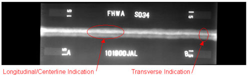
Figure 36. Laboratory specimen S034: Radiographic image showing the two implanted cracks.


The photo shows the plan view of laboratory specimen S034 with the weld oriented horizontally. The left and right sides of the specimen are labeled A and B, respectively.
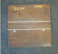
Figure 37. Laboratory specimen S034: Top view of joint.


Figure 38 shows a color-coded image created by the P-scan system which includes the C-scan, B-scan, side view, and response amplitude profile of the weld. The vertical and horizontal axes of the C-scan, B-scan, and side views represent weld dimensions in inches. The vertical and horizontal axes of the amplitude response graph are response amplitude in decibels and distance in inches, respectively. The P-scan image also contains a bar graph relating response magnitude to a series of colors. The colors range from red, which indicates a high amplitude response, to purple, which indicates a low amplitude response. The display clearly identifies the centerline crack but not the transverse crack.
Figure 38. P-scan images of laboratory specimen S034: Images of longitudinal/centerline indication in the weld.

The photo shows a plan view of laboratory specimen S125. The weld is oriented horizontally and aligned with the Y-axis. The X-axis is aligned with the left side of the specimen. The areas above and below the Y-axis are labeled TSC and BSC, respectively.
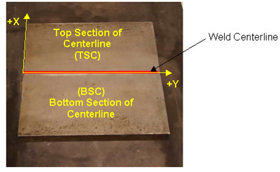
Figure 39. Laboratory specimen S125: Top view of joint.


The radiographic image shows two longitudinal cracks along the weld length. The cracks are circled in black for illustrative purposes.
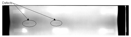
Figure 40. Laboratory specimen S125: Radiographic image showing discontinuities in the weld.

Figure 41 shows a color-coded image created by the P-scan system which includes the C-scan, B-scan, side view, and response amplitude profile of the weld. The vertical and horizontal axes of the C-scan, B-scan, and side views represent weld dimensions in inches. The vertical and horizontal axes of the amplitude response graph are response amplitude in decibels and distance in inches, respectively. The P-scan image also contains a bar graph relating response magnitude to a series of colors. The colors range from red, which indicates a high amplitude response, to purple, which indicates a low amplitude response. The display clearly identifies two longitudinal cracks along the weld length.
Figure 41. P-scan images of laboratory specimen S125: From TSC side of centerline.

This figure shows a color-coded image created by the P-scan system which includes the C-scan, B-scan, side view, and response amplitude profile of the weld. The vertical and horizontal axes of the C-scan, B-scan, and side views represent weld dimensions in inches. The vertical and horizontal axes of the amplitude response graph are response amplitude in decibels and distance in inches, respectively. The P-scan image also contains a bar graph relating response magnitude to a series of colors. The colors range from red, which indicates a high amplitude response, to purple, which indicates a low amplitude response. The display clearly identifies three longitudinal cracks along the weld length.
Figure 42. P-scan images of laboratory specimen S125: From BSC side of centerline.

The photo shows a plan view of laboratory specimen S126 with the weld oriented horizontally.
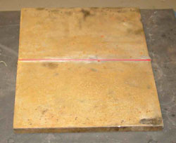
Figure 43. Laboratory specimen S126: Top view of joint.


The radiographic image shows three longitudinal discontinuities along the weld length. The discontinuities are circled for illustrative purposes.
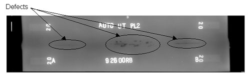
Figure 44. Laboratory specimen S126: Radiographic image showing discontinuities in the weld.

Figure 45 shows a color-coded image created by the P-scan system which includes the C-scan, B-scan, side view, and response amplitude profile of the weld. The vertical and horizontal axes of the C-scan, B-scan, and side views represent weld dimensions in inches. The vertical and horizontal axes of the amplitude response graph are response amplitude in decibels and distance in inches, respectively. The P-scan image also contains a bar graph relating response magnitude to a series of colors. The colors range from red, which indicates a high amplitude response, to purple, which indicates a low amplitude response. The display clearly identifies three rejectable indications along the weld length.
Figure 45. P-scan images of laboratory specimen S126: From TSC side of centerline.

Figure 46 shows a color-coded image created by the P-scan system which includes the C-scan, B-scan, side view, and response amplitude profile of the weld. The vertical and horizontal axes of the C-scan, B-scan, and side views represent weld dimensions in inches. The vertical and horizontal axes of the amplitude response graph are response amplitude in decibels and distance in inches, respectively. The P-scan image also contains a bar graph relating response magnitude to a series of colors. The colors range from red, which indicates a high amplitude response, to purple, which indicates a low amplitude response. The display clearly identifies three rejectable indications along the weld length.
Figure 46. P-scan images of laboratory specimen S126: From BSC side of centerline.

The photo shows a plan view of laboratory specimen S132 with the weld oriented vertically.
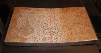
Figure 47. Laboratory specimen S132: View of joint.


The radiographic image does not show any rejectable discontinuities along the weld length.
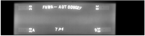
Figure 48. Laboratory specimen S132: Radiographic image showing discontinuities in the weld.

Figure 49 shows a color-coded image created by the P-scan system which includes the C-scan, B-scan, side view, and response amplitude profile of the weld. The vertical and horizontal axes of the C-scan, B-scan, and side views represent weld dimensions in inches. The vertical and horizontal axes of the amplitude response graph are response amplitude in decibels and distance in inches, respectively. The P-scan image also contains a bar graph relating response magnitude to a series of colors. The colors range from red, which indicates a high amplitude response, to purple, which indicates a low amplitude response. The display clearly identifies three rejectable indications between 0 and 177.8 millimeters (0 and 7 inches) from the datum. Note that 1 inch equals 25.4 millimeters.
Figure 49. P-scan images of laboratory specimen S132: From TSC side of centerline between 0 and 177.8 mm (0 and 7 inches).


Figure 50 shows a color-coded image created by the P-scan system which includes the C-scan, B-scan, side view, and response amplitude profile of the weld. The vertical and horizontal axes of the C-scan, B-scan, and side views represent weld dimensions in inches. The vertical and horizontal axes of the amplitude response graph are response amplitude in decibels and distance in inches, respectively. The P-scan image also contains a bar graph relating response magnitude to a series of colors. The colors range from red, which indicates a high amplitude response, to purple, which indicates a low amplitude response. The display clearly identifies three rejectable indications between 0 and 177.8 millimeters (0 and 7 inches) from the datum. Note that 1 inch equals 25.4 millimeters.
Figure 50. P-scan images of laboratory specimen S132: From BSC side of centerline between 0 and 177.8 mm (0 and 7 inches).


Figure 51 shows a color-coded image created by the P-scan system which includes the C-scan, B-scan, side view, and response amplitude profile of the weld. The vertical and horizontal axes of the C-scan, B-scan, and side views represent weld dimensions in inches. The vertical and horizontal axes of the amplitude response graph are response amplitude in decibels and distance in inches, respectively. The P-scan image also contains a bar graph relating response magnitude to a series of colors. The colors range from red, which indicates a high amplitude response, to purple, which indicates a low amplitude response. The display clearly identifies three rejectable indications between 177.8 and 304.8 millimeters (7 and 12 inches) from the datum. Note that 1 inch equals 25.4 millimeters.
Figure 51. P-scan images of laboratory specimen S132: From TSC side of centerline between 177.8 and 304.8 mm (7 and 12 inches).


Figure 52 shows a color-coded image created by the P-scan system which includes the C-scan, B-scan, side view, and response amplitude profile of the weld. The vertical and horizontal axes of the C-scan, B-scan, and side views represent weld dimensions in inches. The vertical and horizontal axes of the amplitude response graph are response amplitude in decibels and distance in inches, respectively. The P-scan image also contains a bar graph relating response magnitude to a series of colors. The colors range from red, which indicates a high amplitude response, to purple, which indicates a low amplitude response. The display clearly identifies three rejectable indications between 177.8 and 304.8 millimeters (7 and 12 inches) from the datum. Note that 1 inch equals 25.4 millimeters.
Figure 52. P-scan images of laboratory specimen S132: From BSC side of centerline between 177.8 and 304.8 mm (7 and 12 inches).


The photo shows a plan/side view of laboratory specimen S133 with the weld oriented vertically.
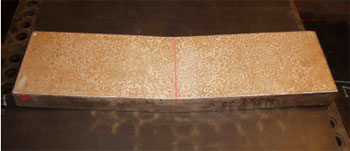
Figure 53. Laboratory specimen S133: Top view of joint.

The radiographic image does not show any rejectable discontinuities along the weld length.Figure 54. Laboratory specimen S133: Radiographic image showing discontinuities in the weld.


Figure 55 shows a color-coded image created by the P-scan system which includes the C-scan, B-scan, side view, and response amplitude profile of the weld. The vertical and horizontal axes of the C-scan, B-scan, and side views represent weld dimensions in inches. The vertical and horizontal axes of the amplitude response graph are response amplitude in decibels and distance in inches, respectively. The P-scan image also contains a bar graph relating response magnitude to a series of colors. The colors range from red, which indicates a high amplitude response, to purple, which indicates a low amplitude response. The display clearly identifies three rejectable indications.
Figure 55. P-scan images of laboratory specimen S133.


The photo shows a side view of laboratory specimen S135 with the weld oriented vertically. The specimen is comprised of a thicker plate on the left and a thinner plate on the right.
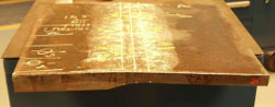
Figure 56. Laboratory specimen S135: Side view of joint.


The photo shows a plan view of laboratory specimen S135 with the weld oriented horizontally. The specimen is comprised of a thicker plate to the top and a thinner plate to the bottom of the photo.
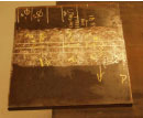
Figure 57. Laboratory specimen S135: Top view of joint.
Previous    Table of Contents    Next


Federal Highway Administration | 1200 New Jersey Avenue, SE | Washington, DC 20590 | 202-366-4000
Turner-Fairbank Highway Research Center | 6300 Georgetown Pike | McLean, VA | 22101