• Federal Highway Administration >
• Publications >
• Research Publications >
• 05063 >
• Chapt8.Cfm >
• Evaluation of LS-DYNA Concrete Material Model 159

Evaluation of LS-DYNA Concrete Material Model 159

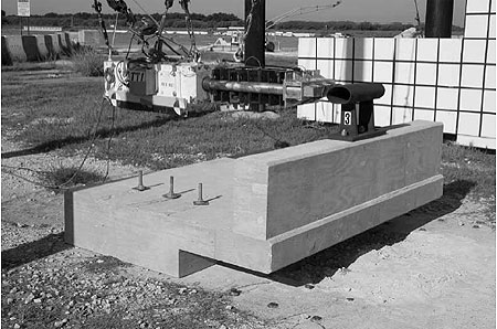
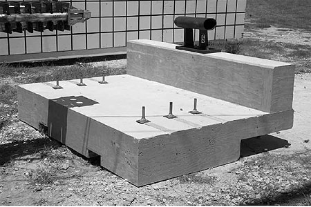
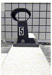
PDF files can be viewed with the Acrobat® Reader®

User Introduction

This chapter, parts of chapter 9, and appendix A present findings related to the evaluation of the concrete material model by a potential end user of the model. The evaluation consisted of a series of verification calculations and validation analyses using the LS-DYNA implementation of the concrete material model (MAT type 159 or MAT_CSCM). The user obtained a beta binaries release of LS-DYNA version 971 for the following platforms: Silicon Graphics, Inc. (SGI) IRIX^® (version 971 release 1490 double precision), MS-Windows (version 971 release 1612 single precision), and Linux Intel 32 bit architecture (version 971 release 1708 single precision). Because LS-DYNA version 971 is a beta release, several releases of these binaries were added during the project period. The research team used the Linux Intel 32 bit architecture (version 971 release 1708 single precision) release to maintain consistency and avoid potential software glitches associated with beta releases that occurred subsequent to the project's initiation.

The work plan followed in the model evaluation process consisted of two tasks. First, calculations were performed to establish that the executable of LS-DYNA obtained by the user gave the same results as the executable used by the developer. This was accomplished by reproducing five developer evaluation calculations using developer-supplied input files. The calculations included three concrete impact simulations that correlate with bogie impact tests of reinforced concrete beams, and two drop-tower simulations that correlate with drop-tower tests. Results of these calculations are given in appendix A.

Second, the concrete material model was used in the impact analysis of a roadside safety structure in which some concrete failure was observed. The structure selected for analysis was the Texas T4 bridge rail. After the initial evaluation of the concrete material model, the roadside safety structure model was used in a parametric study to evaluate model sensitivity to variations in key material parameters. Results of calculations conducted by the user are given in this chapter . Additional support calculations conducted by the developer are given in appendix B.

The user wanted to more fully evaluate the concrete material model in other roadside safety structures. Considerable test data exist for various bridge rail parapets, bridge decks supporting metal rails, and portable concrete barriers in which varying degrees of concrete damage and/or failure occurred. However, the resources allocated for the evaluation and validation effort were not sufficient to support additional model development and analyses. A model of a safety-shape bridge rail with New Jersey profile was developed under this research effort. Data available for this bridge rail included quasi-static load tests to failure and two full-scale vehicular crash tests. Although some preliminary calculations were performed on this model, project resources were depleted before the structure could be fully analyzed by the user. Preliminary calculations performed by both the user and developer are discussed in chapter 9.

Overview

This task involved modeling and analyzing a roadside safety structure made of concrete and using the results to help define the applicability of the concrete material model to the analysis and design of concrete roadside safety structures. The structure selected for analysis was the Texas Type T4 bridge rail.

Two different design variations of the T4 rail were evaluated through dynamic pendulum testing under a previous research study.⁽¹²⁾ Using these tests for evaluation of the concrete model has several benefits. First, the tests provide an opportunity to assess the concrete model in a roadside safety application. Second, use of the pendulum bogie makes the tests more controlled and eliminates the variability associated with full-scale vehicles. Third, two specimens were tested for each design variation, which provides some information about system variability. Finally, the two design variations demonstrated different levels of damage and, therefore, provide the ability to assess sensitivity of the concrete model to small design changes under similar loading conditions.

Pendulum Testing

The T4 railing consists of a 381-mm- (15-inch-) tall metal rail anchored to the top of a 457.2-mm- (18-inch-) tall concrete parapet wall, providing an overall rail height of 838.2 mm (33 inches). The metal rail consists of a short section of an elliptically shaped steel tube welded atop a post fabricated from steel plate. The steel post is welded to a steel base plate that is anchored to the concrete parapet.

In one design variation, the width of the steel-reinforced concrete parapet is 254 mm (10-inch), and the steel rail is attached to the parapet using four 22.2-mm- (0.087-inch-) diameter anchors. In the second variation, the width of the concrete parapet is 317.5 mm (12.5 inches), and the steel rail is attached to the parapet using three 22.2-mm- (0.087-inch-) diameter anchors. Vertical reinforcement in the parapets consisted of #5 V bars spaced 266.7 mm (10.5 inches) apart. Longitudinal reinforcement in the parapets consisted of two #5 bars equally spaced at the top of each parapet and within the V bars.

Detailed drawings of the bridge rail specimens are shown in Figures 83 and 84 for the 254-mm- (10-inch-) and 317.5-mm- (12.5-inch-) wide parapet designs, respectively. A photograph of a test specimen with a 254-mm- (10-inch-) wide parapet is shown in Figure 85; a photograph of the test installation with a 317.5-mm- (12.5-inch-) wide parapet is shown in Figure 86.

To simulate the actual connection of the rail system to a bridge, each parapet was constructed on top of a 203.2-mm- (8-inch-) thick steel-reinforced concrete bridge deck that was cantilevered off a concrete beam a distance of 736.5 mm (29 inches). Transverse reinforcement in the deck cantilevers consisted of two layers of #5 bars located 152.4 mm (6 inches) apart. Longitudinal reinforcement in the top layer of each deck consisted of #4 bars located 228.6 mm (9 inches) apart. Longitudinal reinforcement in the bottom layer of the deck cantilevers consisted of two #5 bars located near the field side edge spaced approximately 76.2 mm (3 inches) apart with the next adjacent bar located 304.8 mm (12 inches) away. Average concrete compressive strengths for the decks and parapets were determined on the day of testing to be:

• 35.50 MPa (5,149 lbf/inch²) for the decks for all tests.
• 30.44 MPa (4,415 lbf/inch²) for the parapets for all tests.

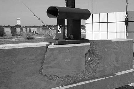
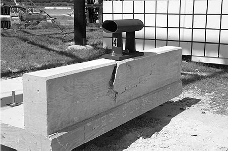
Test Results

Testing was conducted with a gravitational pendulum equipped with a crushable nose assembly. The pendulum bogie was built in accordance with the specifications of the Federal Outdoor Impact Laboratory's (FOIL) pendulum. The crushable nose assembly is the FOIL 10-stage honeycomb nose that uses expendable aluminum honeycomb material of differing densities in a sliding frame structure. Frontal crush stiffness of the staged nose assembly is calibrated to represent the frontal crush stiffness of a small passenger car. The pendulum body was instrumented with an accelerometer. The mass of the instrumented pendulum bogie was 838 kg (1,848 lb), and it was raised to a height sufficient to achieve an impact speed of 9,835 mm/sec, (387.2 inches/sec), which is 35.4 km/h (22 mi/h)). The nose of the pendulum bogie contacted the elliptical tube on the steel rail portion of the system. The impact loads were transferred to the concrete parapet and deck through the steel rail.

For each design variation of the T4 bridge rail, two identical specimens were constructed and tested. For the design variation with the 254-mm- (10 inch-) wide parapet, the test designations were P3 and P4. For the design variation with the 317.5-mm- (12.5-inch-) wide parapet, the test designations were P5 and P7.

The observed failure mode in tests P3 and P4 was punching shear failure of the field side of the concrete parapet due to load applied through the anchor bolts and base plate. In each test, the impact forces caused the concrete to fracture and spall off the field side of the parapet. In addition, cracks in the top of the concrete parapet radiated outward from the outside anchor bolts of the base plate and pieces of concrete were pushed out on the field side of the parapet. Damage to the test specimen with a 254-mm- (10 inch-) wide parapet after test P3 is shown in Figure 87. Post-test damage from test P4 is shown in Figure 88.

mm = 0.039 inch

Figure 83. Details of T4 rail with four-bolt anchorage and 254-mm- (10-inch-) wide parapet.

mm = 0.039 inch

Figure 84. Details of T4 rail with three-bolt anchorage and 317.5-mm- (12.5-inch-) wide parapet.

Figure 85. Parapet before test P3.

Figure 86. Parapet before test P5.

Figure 87. Parapet damage after test P3.

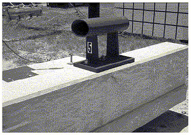
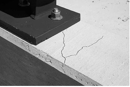
Figure 88. Parapet damage after test P4.

In test P5, a T4 rail with three-bolt anchorage design and a 317.5-mm- (12.5-inch-) wide parapet was evaluated. The pendulum impact caused no visible damage to the concrete parapet or deck. Damage to the test specimen with a 317.5-mm- (12.5-inch-) wide parapet after test P5 is shown in Figures 89 and 90. The same parapet was tested again (test P6) with different staging of the pendulum nose assembly. The impact caused small cracks to be formed in the concrete parapet. The cracks radiated out at an angle from the anchor bolts on the top of the parapet and continued at an angle down the field side of the parapet into the bridge deck.

The second test specimen with 317.5-mm- (12.5-inch-) wide parapet was evaluated in test P7. The impact conditions and pendulum configuration were the same as those used in tests P3, P4, and P5. The impact forces imparted by the pendulum caused the formation of thin hairline cracks in the top of the concrete parapet that radiated out from the anchor bolts of the base plate and down the field side of the parapet into the bridge deck. Post-test damage from test P7 is shown in Figure 91.

Simulation Methodology

The methodology followed to model the bridge parapets, simulate pendulum impacts, and evaluate the concrete material model consisted of the following steps:

1. Modify, optimize, and calibrate the crushable nose pendulum model.
2. Construct finite element model of the two variants of the T4 rail system.
3. Incorporate the new concrete material model for concrete parts (e.g., parapet and bridge deck).
4. Identify critical parameters of the model and investigate the performance of the model through finite element analysis.
5. Compare results with test data and identify any further investigation needed.

Pendulum Model Calibration

To simulate the test conditions described here, it is critical to have an accurate representation of the impacting device. A model of the FOIL pendulum with crushable honeycomb nose assembly was obtained from NCAC. The internal honeycomb cartridges and spacers comprising the nose of the pendulum (see Figure 92) were replaced with a single nonlinear spring as shown in Figure 93. The external honeycomb cartridge on the leading edge of the nose assembly was maintained in the model. However, its density was increased to account for mass of the removed cartridges. Previous experience with the original model with honeycomb nose required runtimes of around 8 central processing unit hours on a mainframe computer to complete a calibration run with the pendulum impacting a rigid pole. The modified pendulum model requires only 15 minutes on a personal computer for a similar problem. The spring-based pendulum (SBP) model was calibrated using a test of the pendulum impacting a rigid pole. The stiffness values of the nonlinear spring were iteratively adjusted until the force-time history obtained from the SBP model closely matched data measured in the rigid pole test.⁽¹³⁾

Figure 89. Parapet damage after test P5, side.

Figure 90. Parapet damage after test P5, rear.

Figure 91. Parapet damage after test P7.

Figure 92. Original pendulum model.

Figure 93. Modified pendulum model.

As shown in Figure 94, the SBP model's force-time history closely matches the rigid pole pendulum calibration test. This calibrated model was used in initial simulations of both variations of the T4 bridge rail system. As the research progressed, it was observed that the impact forces imparted by the pendulum model did not correspond to those measured in the pendulum tests. Comparison of the T4 bridge rail test data with the original pendulum calibration test data indicated that the initial segments of the pendulum nose used in the T4 bridge rail tests were stiffer than those used in the original rigid pole calibration tests. Whereas the pendulum response in tests P3, P4, P5, and P7 appeared reasonably consistent, the response measured in the calibration tests differed.

kN = 225 lbf

Figure 94. Comparison of the SBP model to rigid pole calibration test.

Aluminum honeycomb is known to be a variable material. While crush characteristics of the honeycomb used in the rigid pole calibration were quantified through separate axial compression tests, no such tests were performed prior to the T4 bridge rail tests. It is speculated that the crush properties of the honeycomb material used to construct the crushable nose assembly in the 1997 rigid pole calibration tests differed from those of the honeycomb materials used in the 2002 pendulum tests of the T4 bridge rail specimens. Any change in pendulum stiffness would affect the force-time history response and, hence, the energy applied to the barrier.

Because proper load application is critical to evaluating barrier damage and the concrete material model, a recalibration exercise was undertaken. Test P5 on the T4 bridge rail alternative with three-bolt anchorage and 317.5-mm- (12.5-inch-) wide parapet was used for recalibrating the nonlinear spring representing the honeycomb cartridges. This test was selected because no damage to the parapet was observed after the test. However, the rail system did undergo some elastic deformation and rebound during the test. Thus, the calibration process involved applying a prescribed displacement to the elliptical steel rail. The displacements that were prescribed on the rail were obtained from the test using high-speed film analysis measurements. By explicitly accounting for the displacement of the rail, the pendulum response can be uniquely obtained.

As with the original calibration, the recalibration process involved iteratively adjusting the stiffness values of the nonlinear spring model until the resulting force-time history closely matched data measured in the test P5. The recalibrated pendulum model was labeled SBP2. As shown in Figure 95, the pendulum configuration used in the rigid pole test has a different force-time history than the pendulum used in the test of the almost rigid T4 rail with 317.5-mm- (12.5-inch-) wide parapet (test P5). The good correlation achieved between the recalibrated pendulum model (SBP2) and the pendulum configuration used in test P5 can also be observed in Figure 95.

Figure 96 presents the force-deflection relationships obtained from both simulation and testing of both the rigid pole and T4 bridge rail with 317.5-mm- (12.5-inch-) wide parapet (test P5). As shown in this figure, the crushable nose used in test P5 is indeed stiffer than that used in the original rigid pole pendulum calibration test. It can also be observed from Figure 96 that the recalibrated pendulum model provides reasonable correlation with the pendulum used in test P5. The pendulum model follows the same stiffness trend, and the difference in energy between simulation and test is less than 1.0 percent.

N = 225 lbf

Figure 95. Force-time histories for benchmark tests and spring models.

kN = 225 lbf

Figure 96. Force-displacement relationships for benchmark tests and SBP2 model.

Finite Element Model of T4 Bridge Rail

Finite element analysts typically follow certain procedures before and after running the numerical solver to help maintain quality control and achieve efficient analysis. The solver used for this study was LS-DYNA. LS-DYNA is an explicit-implicit, multiphysics, nonlinear finite element solver. The pre-processor used for this study was HyperMesh^®. The post-processor used was LS-POST. The following steps were followed in analyzing the application of the new concrete material model in the T4 bridge rail system:

1. Geometrical modeling of the structure's components. This step includes defining the spatial topology of the model.
2. Meshing the model. In this step, the spatial topology of each model component is discretized into thousands of small elements (i.e. finite elements).
3. Defining sectional properties. This step includes establishing the thickness of shell elements, the cross-sectional properties of beam elements, and prescribing an element formulation for all element types.
4. Prescribing boundary conditions, contacts, initial velocity, and other constraints needed for accurately representing the physics of the impact.
5. Incorporating material models for all parts including concrete components.
6. Conducting the analysis.
7. Post-process results and comparing these results to test data.

Various steps of this process were systematically repeated to evaluate sensitivity of the model's response to changes in certain modeling and material parameters.

Overview of T4 Parapet/Deck Model

The finite element representation of the T4 bridge rail specimens consists of the following components:

• Concrete parapet and deck.
• Steel reinforcement and anchor bolts.
• Steel elliptical rail, post, and base plate.

Figures 97 and 98 show the model components for the four-bolt and three-bolt parapet designs, respectively. The concrete parapet and bridge deck were modeled using solid elements, as were the steel base plate and the plates comprising the steel post. Shell elements were used to model the elliptical steel rail. Beam elements were used to model the anchor bolts and steel reinforcement inside the parapet and bridge deck.

Figure 99 shows a closeup view of the steel portion of the bridge rail model, including the elliptical rail, post, base plate, and anchor bolts. Figures 100 and 101 show the steel reinforcement and anchor bolts incorporated into the four-bolt and three-bolt parapet models, respectively. All vertical and longitudinal steel were explicitly modeled.

Figure 97. Model of T4 bridge rail specimen with four-bolt anchorage and 254-mm- (10-inch-) wide parapet.

Figure 98. Model of T4 bridge rail specimen with three-bolt anchorage and 317.5-mm- (12.5-inch-) wide parapet.

Figure 99. Closeup view of steel rail system with four-bolt anchorage.

Figure 100. Steel reinforcement and anchor bolts for T4 bridge rail specimen with four-bolt anchorage and 254-mm- (10-inch-) wide parapet.

Figure 101. Steel reinforcement and anchor bolts for T4 bridge rail specimen with three-bolt anchorage and 317.5-mm- (12.5-inch-) wide parapet.

Figure 102. Right end view of parapet-only model for four-bolt design and three-bolt design.

The investigations included evaluating model sensitivity to variations in material parameters and making any needed changes to the default values coded into the material model subroutine. To facilitate this effort and reduce the computational time required to perform numerous parametric runs, the parapet models were extracted from the bridge rail system models as shown in Figure 102. The bottom edge of the parapet in these subsystem models was constrained against movement. Although this artificially increased the stiffness of the parapet to some degree, it provided a more computationally efficient means of evaluating the effect of model changes on parapet response. After converging on a reasonable set of parameters, the full system models (including bridge deck) were simulated and the results compared to measured and observed test data.

Meshing

As indicated previously, the concrete parts were meshed with solid elements, the steel base plate and post were meshed with solid elements, the tubular rail element was meshed using shell elements, and the steel reinforcement and anchor bolts were meshed using beam elements. The meshes for these components were kept fixed during this study except for the mesh of the concrete parapet.

The original mesh of the parapet was constructed to enforce matching between nodes of concrete and those of the steel reinforcement. This construction enables coincident nodes to be merged, thus ensuring connectivity between the concrete and steel components. This parapet mesh is depicted in Figure 103. Together, the concrete parapet and deck models had a total of 115,000 elements. The requirement of matching nodes led to elements with poor aspect ratios and the creation of unnecessarily small element sizes (e.g., 7 mm (0.276 inch) and 5.6 mm (0.22 inch)), which has a significant effect on time step control.

To mitigate this problem, a different connection scheme was utilized between the parapet and the steel reinforcement, which permits a more regular, uniform mesh to be used throughout the parapet. Use of coupling (*CONSTRAINED_LAGRANGE_IN_SOLID) permits the concrete mesh to be assigned without consideration of the location of steel reinforcement. Details of this connection scheme are explained in the Constraints and Boundary Conditions section of this report.

A uniform mesh of 25.4-mm (1-inch) solid elements was used in some preliminary calculations. However, an alternate meshing strategy with a biasing scheme was ultimately used in the evaluation to provide desired refinement in critical areas of the model without significantly affecting the overall size and run time of the model. A two-dimensional biasing scheme was incorporated into the model of the concrete parapet. Along the parapet height, the elements were linearly biased from approximately 20 mm (0.79 inch) at the bottom of the parapet to 13 mm (0.51 inch) at the top of the parapet using a linear biasing function in HyperMesh. A bell curve biasing was used along the length of the parapet with element sizes ranging from approximately 36 mm (1.42 inches) at the ends of the parapet to 16 mm (0.63 inch) in the middle of the parapet. The meshing across the width of the parapet was kept semi-uniform with an element size of 16 mm (0.63 inch). Thus, the largest solid element in the parapet was 16 mm (0.63 inch) by 20 mm (0.79 inch) by 36 mm (1.42 inches); the smallest was approximately 14-mm by (0.55 inches) by 13 mm (0.51 inch) by 16 mm (0.63 inch). A cross section of the revised parapet mesh is shown in Figure 104.

The bridge deck was meshed uniformly along its length using an element size of 25.4 mm (1 inch). A linear biasing technique was used across the width of the deck (i.e., along the impact direction), with larger elements used at the front deck and smaller elements used at the back of the deck where it ties into the parapet. The biased meshing scheme used for the parapet and deck system, which consists of approximately 76,000 elements, is shown in Figures 105 and 106.

Sectional Properties

The thickness for the shell elements comprising the elliptical steel rail and the cross-sectional properties of the beam elements used to model the steel reinforcement and anchor bolts were assigned according to the details and specifications of the Texas Type T4 bridge rail system. Fully integrated elements (type 16) were used for the steel rail, and the Hughes-Liu beam element with cross section integration (type 1) was used for the steel reinforcement and anchor bolts. The concrete brick elements were type 1 (underintegrated) with stiffness form of hourglass control (type 5) specified.

Constraints and Boundary Conditions

For cases in which the bridge deck was included in the analysis, the constraints were imposed on the front side of the deck and beam, the bottom of the beam, and the ends of the transverse steel reinforcement in the deck as shown in Figure 107. In the simulations conducted with the parapet-only subsystem, the bottom of the parapet and the lowermost points of the vertical reinforcement were constrained (i.e., fixed) in all degrees of freedom. Figure 107 also shows an illustration of the boundary condition setup for this case.

Boundary conditions were also imposed on some of the nodes of the rigid pendulum body to constrain the motion of the pendulum body in both the vertical and the lateral directions (both of which are perpendicular to the impact direction). Motion of the pendulum in these two directions is limited by the cables attaching the pendulum to its support towers. Note that the pendulum follows a circular arc. Thus, the linear motion prescribed is an approximation, which is accurate within a small displacement setting as is the case with the T4 bridge rail.

A constraint was used to represent the interaction between the anchor bolts, steel reinforcement, and the surrounding concrete continuum. The steel reinforcement and anchor bolts are coupled (rather than merged) to the surrounding concrete continuum. This coupling was achieved using the *CONSTRAINED_LAGRANGE_IN_SOLID feature in LS-DYNA. In this constraint, the steel reinforcement and anchor bolts are treated as slave material that is coupled with a master material comprised of the deck and parapet concrete. Using this methodology, the slave part(s) can be placed anywhere inside the master continuum part without any special mesh accommodation.

Figure 103. Original parapet mesh used for merging nodes with steel reinforcement.

Figure 104. Revised parapet mesh with steel reinforcement.

Figure 105. Linear mesh biasing along the height of parapet and width of deck.

Figure 106. Bell curve mesh biasing along length of parapet and uniform meshing along length of deck.

Figure 107. Boundary conditions used for the full system model with deck and for the parapet-only model.

To verify the proper functionality of this method, an example of a reinforced concrete beam modeled with merged nodes as supplied by the developer was modified and rerun using the coupling methodology. The response and damage obtained for the two runs was very close.

The anchor bolts are also constrained to the steel base plate via node merging. Each bolt is merged to one node on the upper surface and one node on the lower surface of the base plate. This constraint is illustrated in Figure 108.

Figure 108. Anchor bolt constraint to base plate.

Three contacts were defined within the bridge parapet model to account for interactions between various components: one between the lower surface of the base plate and the top of the parapet, one between the lower surface of the parapet and the deck, and one for interaction among the steel reinforcement bars. Note that the bridge rail test specimens were constructed using two different concrete pours: one of the deck and one for the parapet. The contact definition between the parapet and deck represents the construction joint that exists between these two components. This contact definition was not used when the parapet-only model was being analyzed.

It is also noteworthy that the pendulum model has its own internal contact definition as well as an additional contact definition between the front cartridge of the crushable nose and the tubular steel rail section. All of these contact definitions are depicted in Figure 109.

Figure 109. Contacts definitions for the T4 bridge rail model.

Material Definitions

Material models are essential to accurately studying the performance of any system. This research focuses specifically on the newly developed concrete material model; however, other material models (e.g., steel) also had to be implemented to achieve appropriate system response. All steel reinforcement was modeled using an elastoplastic material model that incorporates a strain rate effect on yield strength. The anchor bolts were modeled using elastic steel definition due to their size (19.05-mm- (0.75-inch-) diameter), material composition (high strength steel), and the behavior observed in the full-scale pendulum tests. It was analytically verified through careful monitoring of bolt stresses that none of the anchor bolts reached yield stress at any time during simulation. The tubular rail, the base plate, and the steel posts were modeled using an elastoplastic material model definition.

The parapet and deck were both modeled using the new concrete material model developed by APTEK. In the beta version of LS-DYNA 971, it is designated as material type 159. The model name is *MAT_CSCM_CONCRETE or *MAT_CSCM. The "_CONCRETE" suffix indicates a short input format that utilizes hard-coded default values for numerous variables; the other name indicates a long input format for which the user must supply values for all the required input parameters. Input parameters are not listed here because they are explained in the companion Users Manual for the material model. However, some salient parameters studied in this research are discussed. These parameters are (as excerpted from the Users Manual):

ERODE Elements erode when damage exceeds 0.99 and the maximum principal strain exceeds 1 − ERODE. For erosion that is independent of strain, set ERODE equal to 1.0. Erosion does not occur if ERODE is less than 1.0.

f '_C Unconfined compression strength. If left blank, default is 30 MPa (4,351 lbf/inch²).

Dagg Maximum aggregate size. If left blank, default is 19 mm (0.75 inches).

G_fc Fracture energy in uniaxial compression.

G_ft Fracture energy in uniaxial tension.

G_fs Fracture energy in pure shear.

repow Power that increases fracture energy with rate effects.

The element erosion parameter (ERODE) is part of both input formats. The compression strength of concrete (f'_C) and the maximum aggregate size (Dagg) are required as part of the short input format. The fracture energy related parameters (G_fc,G_ft , G_fs, repow) are part of the long input format. The short input format will work with default model parameters based on the user-supplied compression strength of concrete (f '_C) and the maximum aggregate size (Dagg); the long format requires the user to explicitly define all the model parameters.

For the T4 bridge rail analysis, the concrete had a maximum aggregate size of 25.4 mm (1 inch). The concrete used for the bridge deck had an average compressive strength of 35.5 MPa (5,149 lbf/inch²) on the day of testing. The parapet concrete had an average compressive strength of 30.44 MPa (4,415 lbf/inch²).

In this study, the short input format was used to generate and list the full set of parameters in the LS-DYNA output file. These parameters were then used in the long input format, and selected parameters were varied as part of the performance/sensitivity study.

Analyses of T4 bridge Rail

Numerous analyses were conducted using the models of the T4 bridge rail variants as part of the evaluation of the concrete material model. Only the significant analyses are reported here.

Baseline Parameters

All dimensional parameters are based on the following units:

• Megagram for mass.
• Second for time.
• Millimeter for length.
• Newton for force.
• Megapascal for stress or pressure.
• Millijoules for energy.

This corresponds to the UNITS field being set to "2" in the third line of the short input format. For the T4 parapet model, which had an average compressive strength of 30.44 MPa (4,415 lbf/inch²) and a maximum aggregate size of 25.4 mm (1 inch), the short input is shown in t Table 8. For the bridge deck, which had an average compressive strength of 35.5 MPa (5,149 lbf/inch²) and a maximum aggregate size of 25.4 mm (1 inch), the short input is shown in Table 9.

Values for the parameters comprising the long input format of the concrete model were obtained from the d3hsp (ASCII output) file of LS-DYNA. However, when these values were obtained, it was noticed that the printed output did not correspond to the format provided in the draft manual. This identification mismatch affected the parameters K, G (modulus), alpha, theta, lambda, and beta of all three surfaces (triaxial compression, torsion, and triaxial extension as well as R and X0. These format errors were communicated to the developer, and corrections were made for later releases of LS-DYNA 971 to make the manual consistent with the output routine.

To avoid any confusion or possible modeling errors, the long format input parameters for the concrete material models used in the analyses of the T4 bridge rail alternatives were submitted to the developer for a correctness check. The long input format parameters for the parapet and deck concrete are shown in Table 10, respectively. The values shown in these tables are herein referred to as the "baseline values." Changes to the material model were made with reference to these baseline values. The parameters that were varied as part of the material model evaluation are shown as shaded. Note that these baseline values are not the default values currently implemented in ls-dyna version 971. They are preliminary values that were later adjusted based on results of all calculations presented within this evaluation report.

Baseline Analysis

A dynamic pendulum impact into the T4 bridge rail with four-bolt anchorage and 254-mm- (10-inch-) wide parapet was simulated using the aforementioned baseline values for the concrete material model and the initial SBP pendulum model. As shown in Figure 110, the damage fringe obtained from the simulation approximates that observed during the testing (see Figure 88). The damage fringes depict the damage of each element on a scale from 0 to 1 where the value 0 indicates no damage and the value 1 indicates total damage (i.e., the element is not capable of carrying load). However, unlike the tests, no material failure (i.e., element erosion) was observed in this simulation.

Figure 110. Damage fringe for baseline simulation of T4 with four-bolt anchorage and 254-mm- (10-inch-) wide parapet.

Parametric Analyses

Given that the baseline values did not provide the desired failure response, a sensitivity study was conducted to investigate system sensitivity to selected parameters. Another analysis (case02) was conducted for which erosion was enabled independent of strain (i.e., ERODE equal to 1.0). The other variables were unchanged from their baseline values.

As shown in Figures 111 and 112, elements were eroded from both the parapet and the deck. With ERODE set to 1.0, the elements eroded based on a set damage threshold (i.e., above 0.99) without consideration of strain. Damage fringes for this simulation case are shown in Figure 113.

Figure 111. Element erosion profile (simulation case02, ERODE =1) on traffic side.

Figure 112. Element erosion profile (simulation case02, ERODE =1) on field side.

Figure 113. Damage fringes for simulation case02 (ERODE =1).

Elements eroded on the field side of the parapet (see Figure 112) propagated in a pattern similar to that observed in the test. However, element erosion on the traffic face of the parapet and the tension (top) face of the bridge deck (see Figure 111) does not replicate test results. Recall that no visible damage or cracks were observed on either of these faces after tests P3 or P4. This result indicates that element erosion should not be used independent of a maximum principal strain criterion.

Another simulation was conducted with the value of the ERODE parameter set to 1.05. Although the pattern of the damage fringes was generally consistent with that observed in the pendulum tests, no element erosion/failure occurred, which makes the results similar to those from the baseline simulation with ERODE = 1.1.

The focus then shifted toward studying the effect of the fracture energies (G_fc, G_fs, and G_ft) on the damage profile and erosion of elements. Initially, very low values of the fracture energies (20 percent of the original baseline values) were used. As might be expected, this change resulted in extensive element erosion and very weak parapet response as shown in Figure 114.

It was noticed during this simulation that the energy balance of the model changed during the analysis. More specifically, the total energy of the system increased. The change was attributed to an inappropriate increase in total internal energy of the system. Further investigation revealed that this unrealistic increase in energy, shown in Figure 115, was traceable to the concrete material. Beginning at about 0.05 s, the total energy increases 2.5 times its original value. The changes in the internal energy of the concrete material correspond to this change in the total system energy and appear to be related to the damage calculations. As damage of the concrete components increases (as indicated by the damage fringes and contours), the total system energy increases.

Similar behavior was present in the baseline simulation as well. However, this behavior was not as readily detectable because the percentage of increase in energy is related to the damage induced in the concrete. This behavior was disclosed to the developer during the early stages of model validation, and a fix was incorporated into later releases of LS-DYNA version 971.

Continuing with the parametric evaluation, the values of fracture energies were next increased to 50 percent of the baseline values. As shown in Figure 116, the associated fracture profile radiated out from the outer anchor bolts on the top of the parapet but did not extend to the field side of the parapet.

A process of bisection of fracture energy values was followed until a set of values that produced a similar fracture profile to that observed in the test was identified. With the fracture energy values set at 27.5 percent of their baseline values, the simulation resulted in a damage pattern and fracture profile similar to those observed in the test. The fracture profile shown in Figure 117 indicates that a piece of concrete similar in shape and size to those that fractured in tests P3 and P4 would fracture and possibly spall off. Additionally, the model captures the deflection and rotation of the anchor bolts inside the parapet wall similar to that observed in the tests.

Figure 114. Parapet failure with fracture energies at 20 percent of baseline values.

Joule = 0.73756 ft-lb

Figure 115. Energy-time histories for pendulum impact of T4 bridge rail with fracture energies at 20 percent of baseline values.

Figure 116. Parapet failure with fracture energies at 50 percent of baseline values.

Figure 117. Parapet failure with fracture energies at 27.5 percent of baseline values.

The energy-time histories associated with this run are shown in Figure 118. As previously discussed, an increase in the total system energy can be observed to coincide with a significant increase in the internal energy of the system at about 0.05 sec. The extent to which the calculations are affected by this behavior is not known. The developer indicated that the problem was confined to a reporting issue and does not affect the simulation outcome. A fix was incorporated into later releases of LS-DYNA version 971.

Realizing that fracture energies set at 27.5 percent of the baseline values could not be physically justified, two other aspects of the model were further investigated. First, in consultation with the developer, the stiffness of the crushable nose of the pendulum impactor was studied to see whether the impact energy absorbed by the pendulum and transferred to the barrier agreed with test data. The second aspect investigated was an enhancement of the anchor bolt connection between the base plate and concrete parapet.

Comparison of data from the rigid pole calibration tests and the T4 bridge rail impacts showed a discrepancy in the stiffness of the nose assembly. Additional checks on the properties of the aluminum honeycomb material commonly used in the crushable nose assembly of the pendulum bogie indicated that the material stiffness can vary considerably (e.g., 10 percent to 20 percent) among different batches. Because the properties of the honeycomb used in the pendulum testing of the T4 bridge rail were not directly measured, a new stiffness curve for the pendulum spring (SBP2) was developed based on test P05 as previously described. The net result is a stiffer pendulum nose that correlates with the honeycomb material used in the actual pendulum tests of the T4 bridge rail systems.

Upon consultation with the developer, it was suggested that a set of fracture energy values at 80 percent of the baseline values is a reasonable lower bound for concrete having a maximum aggregate size consistent with that used in the T4 bridge rail installations. Consequently, the modified SBP2 pendulum model was used in an impact analysis of the T4 parapet system with four-bolt anchorage and 254-mm- (10-inch-) wide parapet using 80 percent of the baseline fracture energy values. However, this configuration did not result in a significant change to the damage profile compared with the parapet impacted by the lower stiffness pendulum (SBP).

Next, further study was devoted to the connection between the base plate and anchor bolts. Initially, nodes on the anchor bolts were merged to corresponding nodes on the base plate. This merging constrained the base plate from rotation, a behavior that was observed in the high-speed video of the pendulum tests. The interaction between the base plate and anchor bolts was subsequently enhanced by removing the merged nodes connection and adding washers on the top surface of the base plate to constrain upward vertical motion of the base plate. The washers were tied to the anchor bolts. A *CONSTRAINED_NODE_SET was added between nodes of the anchor bolts and the closest base plate nodes to constrain motion in the horizontal plane of the base plate.

Joule = 0.73756 ft-lb

Figure 118. Energy-time histories for pendulum impact of T4 bridge rail with fracture energies at 27.5 percent of baseline values.

This configuration gives the base plate more freedom to rotate when subjected to an applied moment due to rail impact based on the material properties of the bolts and washers. The vertical downward constraint on the base plate was handled by contact with the top surface of the concrete parapet. This modeling change was considered to more accurately represent the behavior of the actual connection without significantly affecting computer processing time. The enhanced connection model between the base plate and anchor bolts is depicted in Figure 119.

Figure 119. Enhanced anchor bolt-to-base plate connection model.

Modified System Analyses

An LS-DYNA model was constructed using the SBP2 pendulum model, the lower end of the recommended fracture energy values (80 percent of baseline values), and the enhanced base plate-to-anchor bolt connection. The parapet-only model of the T4 parapet system with four-bolt anchorage and 254-mm- (10-inch-) wide parapet (discussed previously) was used in the simulation to reduce computational time.

Figures 120-122 show sequential views of the simulation at different times. Although the general pattern was similar, the fracture damage profile was more extensive than that observed in the pendulum tests (tests P3 and P4). This result was expected in part due to the use of the parapet-only model, which is less flexible than the more detailed model configuration that incorporates the bridge deck. It is noteworthy that the rail-post-base plate assembly rigidly rotated and subsequently rebounded as observed in the actual pendulum tests.

Figure 120. Fracture profile of modified T4 system at 0.080 seconds.

Figure 121. Fracture profile of modified T4 system at 0.115 seconds.

Figure 122. Fracture profile of modified T4 system at 0.250 seconds.

Full System Analysis: Four-Bolt Design

The parameters used in the analysis of the parapet-only simulation of the modified T4 parapet system with four-bolt anchorage and 254-mm- (10-inch-) wide parapet were incorporated into the full system model that included the bridge deck. As before, the SBP2 pendulum model was used as the impactor.

A profile of the damaged bridge rail system after impact is shown in Figure 123. The fracture profile of the parapet is shown in Figure 124 with the steel components of the parapet removed for better visualization. Due to the inherent flexibility of the bridge deck, the fracture profile of the concrete parapet was less severe than that for the parapet-only model and was similar to that observed in the pendulum tests. Element erosion radiated from the outer anchor bolts and extended to the back edge of the parapet and down the field side of the parapet wall.

Figure 123. Profile of damaged T4 bridge rail system with four-bolt anchorage after pendulum impact.

Figure 124. Fracture profile for T4 bridge rail with four-bolt anchorage for parapet and eroded elements.

As shown in Table 12, the peak impact force in the simulation of the T4 bridge rail system with four-bolt anchorage compares favorably with those measured in the corresponding pendulum tests. Acceleration-time histories for the tests and simulation, filtered at 180 Hertz (Hz), are compared in Figure 125. The simulation data tracks the test data reasonably well up to the time of peak acceleration. After this time, the rebound portion of the pendulum simulation data deviates from the tests. However, this rebound phase does not have direct bearing on the evaluation of the concrete material model or roadside safety structure.

Figure 125. Pendulum bogie accelerations for impact of T4 bridge rail with four-bolt anchorage and 254-mm- (10-inch-) wide parapet.

The peak impact force for test P3 is approximately 10 percent greater than the peak impact force for test P4 and the simulation. Because the test specimens and impact conditions are nominally similar, this difference is attributed to normal material and test variation. The acceleration pulse indicated during the rebound phase of test P3 is attributed to pitching and "bucking" of the suspended pendulum mass.

Figure 126 presents the velocity-time histories for the pendulum tests and simulation. Because these data are based on integration of the acceleration data, they are expected to be smoother and correlate better. Note that the negative portions of the velocity curves represent rebound of the pendulum. The simulation data tracks the data from test P4 up to the rebound phase of the impact (velocity < 0). The data for test P3 deviates from test P4 and the simulation before rebound.

Figure 126. Pendulum bogie velocities for impact of T4 bridge rail with four-bolt anchorage and 254-mm- (10-inch-) wide parapet.

Overall correlation between the simulation and test data is considered to be good. The simulation matches particularly well with test P4. Thus, researchers decided to proceed to simulation of the T4 bridge rail system with three-bolt anchorage and 317.5-mm- (12.5-inch-) wide parapet to further evaluate the concrete material model. When tested, this design variation had a different level of damage than the system with four-bolt anchorage and 254-mm- (10-inch-) wide parapet, thus providing an opportunity to assess the sensitivity of the concrete model to small design changes under similar impact loading conditions.

Full System Analysis: Three-Bolt Design

The same parameters used in the simulation of the T4 bridge rail with four-bolt anchorage and 254-mm- (10-inch-) wide parapet were incorporated into the full system model of the T4 bridge rail with three-bolt anchorage and 317.5-mm- (12.5-inch-) wide parapet. As discussed previously, the full system model incorporates the bridge deck. The modified SBP2 pendulum model was used as the impactor.

Figure 127 shows the calculated response of the parapet-deck system after being impacted by the pendulum. No element erosion occurred in the analysis. The rail/parapet assembly rebounded after a small deflection. Recall that no visible damage was observed after test P5, and only small hairline cracks were found after test P7. Figures 128 and 129 show the damage fringes from the simulation. The fringe pattern is similar to the cracking pattern observed in test P7, which indicates that under a more severe impact, the concrete would fail in a pattern similar to that initiated in test P7.

Figure 127. Profile of T4 bridge rail system with three-bolt anchorage after pendulum impact.

Figure 128. Damage to 317.5-mm- (12.5-inch-) wide parapet after pendulum impact showing element erosion.

Figure 129. Damage to 317.5-mm- (12.5-inch-) wide parapet after pendulum impact showing damage fringes.

The maximum impact force calculated in the simulation compares very favorably with those measured in the test P5 as shown in Table 13. A considerable difference exists between the peak force measured in test P5 and test P7. These tests were conducted on the same day on two different test specimens under nominally similar impact conditions. Beyond test variability, the cause of the difference in peak force is not known.

Acceleration-time histories for the pendulum tests and simulation of the T4 rail system with three-bolt anchorage and 317.5-mm- (12.5-inch-) wide parapet are compared in Figure 130. The simulation data tracks the test data reasonably well during both the loading and unloading (i.e., rebound) phases of the impact. Recall that data from test P5 was used for the recalibration of the pendulum model. Test P7 is an independent test of a similar installation under similar impact conditions. Figure 43 shows that the peak acceleration for test P7 exceeds that for test P5 and the simulation.

Velocity-time histories for the pendulum tests and simulation are presented in Figure 131. The simulation data tracks the test data reasonably well during both the loading and unloading (i.e., rebound) phases of the impact.

Figure 130. Pendulum bogie accelerations for impact of T4 bridge rail with three-bolt anchorage and 317.5-mm- (12.5-inch-) wide parapet.

m/sec = 3.28 ft/sec

Figure 131. Pendulum bogie velocities for impact of T4 bridge rail with three-bolt anchorage and 317.5-mm- (12.5-inch-) wide parapet.

Overall correlation between the simulation and test data is considered to be good. The simulation matches particularly well with test P5 in terms of damage, peak force, and acceleration-time history.

Summary for Bridge Rail Analyses

The analyses of the T4 bridge rail alternatives provided a good benchmark for evaluating the application of the new concrete material model in roadside safety applications. Use of the pendulum bogie provided more controlled tests and eliminated many variables associated with the comparison of simulation to full-scale vehicle crash tests. Two specimens were tested for each design variation, providing some information regarding system variability. Furthermore, the two design variations demonstrated different levels of damage to the concrete parapet, which provided an opportunity to assess the sensitivity of the concrete model to small design changes under similar loading conditions.

After calibration of the material model parameters and enhancement of the base plate connection model, simulations of the two bridge rail alternatives were able to capture the general pattern and severity of concrete damage observed in pendulum tests of both the 254-mm- (10-inch-) and 317.5-mm- (12.5-inch-) wide parapets. As mentioned previously, the user desired to more fully evaluate the concrete material model in other roadside safety structures. A model of a safety-shape bridge rail with New Jersey profile was developed for this purpose. Although some preliminary calculations were performed on this model, project resources were depleted before the structure could be fully analyzed. More details of this bridge rail model, available test data, and discussions of preliminary calculations are presented in the next chapter.

Previous | Table of Contents | Next