U.S. Department of Transportation
Federal Highway Administration
1200 New Jersey Avenue, SE
Washington, DC 20590
202-366-4000
Federal Highway Administration Research and Technology
Coordinating, Developing, and Delivering Highway Transportation Innovations
 |
| This report is an archived publication and may contain dated technical, contact, and link information |
|
Publication Number: FHWA-HRT-06-139
Date: October 2006 |
Representative fluxgate magnetometer installations for various lane configurations are illustrated in Figure 5-53. The probes are buried beneath the roadway surface in cored holes. The optimum depth and placement of the probes depends on the type of detection required (see Chapter 4 and Appendix L) and the size of the probes.
After the preinstallation activities (described earlier in this chapter) have been completed, installation usually follows the step-by-step procedures discussed below.
| 1 ft = 0.3 m |
After securing the work zone with appropriate barricades, cones, etc., to divert traffic from the area, the first step is to layout and mark the detection area with spray paint or chalk markers to match the construction plans. A magnetic field analyzer should be placed over each marked probe location to verify that the area is free of ferrous metal objects that would degrade performance as discussed in Chapter 4.
Holes for the probes are subsequently drilled through the roadway to the proper depth as defined in the construction plans. The general rule for the diameter of the hole is to use the diameter of the sensing probe plus 1/8-inch (3.2 mm).
Slots for the connecting cable are then sawed in the pavement to the adjacent pull box and blown clean and dry with compressed air. The pull box is installed using the same procedures as previously described for loop detectors.
The probe should be installed with the long dimension vertical and with the cable ends at the top. The probe should be firmly supported in the hole so it will not shift from its vertical position.
There are several approaches for placement of the probe in the hole. Manufacturers indicate that the probe is made so that it can be placed in the hole without any protective housing and a number of agencies follow this procedure.
Other agencies prefer to provide some type of housing (e.g., PVC conduit) for placing the probe, while others choose to secure the probe by tightly packing sand or using sealant around it. A representative standard plan for magnetometer installation is shown in Figure 5-54.
| 1 inch = 2.5 cm |
The cables from the probe to the pull box are installed in the sawed slot. A 3/16- to 1/4-in (4.8- to 6.4-mm) wood paddle is used to seat the cable in the sawed slot. A 5-ft (1.5-m) length of extra cable should be left at the pull box. The cables should be identified by lane or by probe designation.
A volt–ohmmeter should be used to verify the series resistance (continuity) of the probe and cable. This value should be the resistance of each probe (4 to 6 ohms per probe) plus the resistance of the cable. The value should be within 10 percent of the calculated value.
Resistance to ground should also be checked. The value should be high, indicating that there are no breaks in the probe or wire insulation. A megger should not be used to check resistance to ground, as the large value of induced voltage will destroy the probe.
Splicing of the sensing element cable to the lead-in cables to the controller cabinet should be soldered using resin core solder. The techniques for splicing are the same as those used for inductive-loop detectors. The lead-in cable should not be spliced between the pull box and the controller cabinet.
The same precautions identified for loop detectors should be addressed when installing magnetometers. Two types of heat-shrinkable polyolefin tubing are used for splicing probe cables to the lead-in (home-run) cable—small diameter tubes insulate the individual conductors and a single large tube seals and protects the splice. An electric heat gun and butane hand torch or electric soldering iron are required to complete the splice. The procedure recommended for splicing probe cables to the lead-in (home-run) cable consists of the steps below:
Each probe element circuit should be tested at the controller cabinet before filling holes and slots. The same measurements described for inductive loop installation should be made using a low range ohmmeter. In this test, the series resistance will be higher because of the added resistance of the lead-in cable.
An operational check should also be conducted at the controller cabinet. Connecting the probe cables to an electronics unit and applying power may accomplish this. The electronics unit should then be calibrated following the manufacturer’s guidelines. Check each probe using a bar magnet oriented in a direction which aids the horizontal or vertical components of the Earth’s magnetic field intensity. Dual-axis fluxgate magnetometers are responsive to horizontal and vertical components of the Earth’s magnetic field. The channel indicator should light up when the bar magnet is located over any probe in the set being tested.
Record the measurements taken. One additional measurement should be made using a yard stick with 1/16-inch (1.6-mm) increment marks and the bar magnet. Stand the yardstick vertically over the probe, place the magnet at the top of the yard stick, and slowly move the magnet down toward the probe until the indicator light on the electronics unit turns on. If the system fails at a later time, the same measurement procedure can be repeated. If the magnet must be closer to the probe to light the indicator, this indicates that the probe has rotated.
Once the system tests are competed, the probe holes and the sawcuts containing the cables can be sealed in the same manner used for inductive-loop detectors. This completes the installation of the magnetometer detector system.
The preinstallation activities for magnetic detectors are much the same as those described for inductive loops. When the magnetic detector probe is installed 12 to 30 inches (30 to 76 cm) under the roadway, the long axis is generally horizontal and is perpendicular to the direction of travel. The conduit, housing the probe, can be installed by either drilling or trenching under the pavement surface as described below.
The preferred method of installation is to tunnel a hole under the pavement from the side of the road and push the conduit into the hole as shown in Figure 5-55. For installation in a four-lane, divided roadway with a median, many agencies have found it desirable to install from the median. The median is preferable as these areas have fewer sign posts, guard rails, and utility activities.
| 1 inch = 2.5 cm |
After locating and marking the desired area for the placement of the probe, measure the distance from the pull box to a point on the road where the conduit ends. Using a backhoe, dig a pit 3 ft (0.9 m) deep, 2 ft (0.6 m) wide, and 10 ft (3 m) long. A horizontal boring machine is then placed in the pit, leveled, squared, and secured. The hole is bored under the pavement, taking care that the drill does not stray from the desired path.
When the drilling is complete, the machine is removed and the pit is backfilled to a level just below the bore hole. A 3- or 4-inch (76- or 102-mm) schedule 40 PVC is capped and placed in the hole, section by section. Each section of pipe must be fitted squarely and glued. Before the final section of PVC is fitted, place the pull box in the trench and set it so that the hole in the box lines up with the pipe. The pipe should fit flush with the wall of the pull box.
Trenching is an alternative to the boring method of installing a conduit to hold the magnetic detector. The first step in this procedure is to mark the boundary of the trench. The pavement is then cut and a trench is excavated including the area for the pull box. A 3- to 4-inch (76- to 102-mm) plastic conduit or fiber duct is laid in the trench and sloped to drain into the pull box in case of water leakage or condensation. The outer end of the conduit should be capped before placing in the trench.
To prevent damage to the probe by the pressure of traffic above it, the conduit should be covered with a minimum of 6 inches (15 cm) of concrete. When dirt or stone covers the conduit, as with macadam roads, the probe should be at least 1 ft (30 cm) below the surface. A sand cushion should be placed immediately below it and above it to prevent stones from being driven into the conduit by impact from the vehicles traveling on the road above.
The probe sensor lead-in wire should be marked when measuring the correct position by laying the probe on the road in the desired position. The mark helps to locate the sensor in the correct position when the wire reaches the edge of the pull box. The sensor is inserted into the conduit and pushed into position using a steel 3/8-inch (9-mm) span wire.
After the probe is placed in the conduit, the next step is to install the pull box in the same way as described for loop detectors. A drain should be provided in the bottom of the box, and the cover should be sealed to prevent the entrance of surface water.
The probe lead-in wire should be spliced to the lead-in cable running to the controller. Because the magnetic detector generates an extremely small current, splices should be soldered. Procedures were discussed previously in this chapter for splicing and environmentally sealing splices used with loopdetector and fluxgate magnetometer installations.
Two conductors are required for each magnetic detector. Since magnetic detectors generate extremely small currents, any size copper wire in the cable is satisfactory. Magnetic-detector circuits should not be run in the same cable sheath with wires carrying traffic signal currents. Leakage between the traffic signal wires and detector wires will cause erratic operation of the detectors. Electromagnetic or electrostatic induction between traffic signal wires and detector wires could cause false calls. However, any number of detector wires can be housed in the same cable sheath without causing interference.
Two tests should be conducted with a volt-ohm meter during installation to determine the series resistance (continuity) and ground resistance. For each probe in the series circuit, the series resistance should register 3,800 ohms, plus or minus 10 percent. If there are two probes, the reading should be approximately 7,600 ohms. If the meter reads several times the normal resistance, a check should be made of the wiring and splicing, and each probe should be tested individually.
Resistance to ground should measure several megohms. Low resistance indicates leakage through the wire insulation or the probe. Such leakage will not prevent relay response unless it is sufficient to reduce the probe output.
When the gain is set on the electronics unit amplifier, it should be at the lowest value possible to insure proper operation. This is done to avoid spurious detection of vehicles in other lanes.
The test readings and gain settings should be recorded on the construction plans and on forms which are stored in the controller cabinet, as well as those filed in the maintenance office. This information should always be referred to when maintenance is required.
Over-roadway sensors require structures such as sign bridges, mast arms, and poles for mounting. If these are not already in place, then appropriate overhead structures must be installed to support the sensors. The field of view or footprint of a sensor, i.e., the area of the roadway within which a vehicle is detected and data are collected by a sensor system, is a function of mounting height, offset of the mounting location from the lanes to be monitored, aperture size, elevation changes, curves, and objects that may block the view. The footprint for many sensor technologies is calculated in a similar manner, with only the aperture, i.e., the active transmitting and receiving area of the sensor, varying. In a microwave sensor, for example, the antenna beamwidth definition utilized to calculate the footprint is the angle in degrees or radians at which the radiated power is reduced by one half (i.e., 3 dB). Ultrasonic sensors use the same beamwidth definition. By contrast, infrared sensors and other optical devices express the beamwidth as the angle at which the first null in the diffraction pattern occurs. In any case, the geometrical relations for the footprint are the same for all these sensor technologies.(16)
The following sections describe representative installation and calibration procedures for video image processor, microwave radar, and laser radar sensors. Sensor manufacturers should be contacted to obtain detailed installation and operating instructions for their products.
Before embarking on an initial large-scale deployment of over-roadway sensors, it is wise to evaluate the performance of the candidate sensors under real-time operating conditions where differences in flow rate, road configuration, obstructions, lighting, and weather can be experienced. Such evaluations have been performed for many of the sensors currently available, but the introduction of new models and the unique features of each deployment location make this requirement a recurring one. Guidelines for conducting such tests are found in the reports issued by several sensor evaluation projects. (See references 17–23.)
Since each site has unique features, distributors of the Autoscope VIP recommend that potential users evaluate candidate sites to determine their suitability for video detection.(24) This site survey assists in developing requirements for lens selection, camera mounting, power and signal transmission, and image processor location.
Site surveys assist in determining whether geometric factors and lack of obstructions near each sensor station allow for the installation of overhead sensors and, if so, what additional mounting structures are required. When wireless transmission of data and video are part of the design, the site survey also determines whether the transmission path between the sensor and data reception locations permits unimpeded transmission.
Questions posed during a site survey include:
Rules of thumb are also available to assist in camera location, mounting, and setup. These are based on the following:
Reports of poor VIP nighttime performance at unlighted intersections at several locations in Indiana led to an investigation into the probable causes of these events.(25,26) The following recommendations were developed by the Indiana DOT (INDOT) with the concurrence of several VIP manufacturers to address these issues:(27)
TXDOT has also developed a manual for deploying video detection at signalized intersections.(28)
The focal length of the lens is dependent on the mounting height of the camera, the local topography, distance to the nearest detection area, and the width of the detection area.(24,29) Some vendors supply a program that calculates the horizontal and vertical fields of view and corresponding focal length of the lens from these input data. If the required focal length does not correspond to a standard lens, then the mounting height or one of the detection area parameters is varied in order to specify a standard lens having a horizontal focal length above or below that of the initial calculation. Table 5-15 shows the horizontal and vertical fields of view for several standard lenses. Some VIP vendors supply variable focal length lenses with their cameras so that a specific lens does not have to be selected in advance. Another advantage of this approach is that the number of different focal length lenses required for maintenance operations is reduced.
| Lens (mm) | 4.8 | 6.0 | 8.0 | 12.5 | 16.0 | 25.0 |
|---|---|---|---|---|---|---|
| Horizontal FOV (deg) | 67.4 | 56.1 | 43.6 | 28.7 | 22.6 | 14.6 |
| Vertical FOV (deg) | 53.1 | 43.6 | 33.4 | 21.7 | 17.1 | 11.0 |
Table 5-16 illustrates how the dimensions of the image area are calculated once the focal length is chosen. A camera mounting height of 40 ft (12.2 m) is assumed.
| Dimension | Symbol | How determined | Value |
|---|---|---|---|
Camera height above detection area |
h | Input parameter | 40 ft (12.2 m) |
Half the vertical angular FOV of the lens |
αV | Lens specification (e.g., from Table 5-11) based on required FOV | 16.7 deg |
Half the horizontal angular FOV of the lens |
αH | Lens specification (e.g., from Table 5-11) based on required FOV | 21.8 deg |
Angle between camera line-of-sight and mounting structure |
θ | θ = (90-5) – αV, where 5 is the number of degrees the FOV is below the horizon | 68.3 deg |
Distance to bottom of image |
d1 | d1 = h tan (θ – αV) | 50.5 ft (15.4 m) |
Width of bottom of image |
w1 | w1 = 2h tan αH /cos (θ – αV) | 51.5 ft (15.7 m) |
Distance to top of image |
d2 | d2 = h tan (θ + αV) 457.2 ft | (139.4m) |
Width of top of image |
w2 | w2 = 2h tan αH /cos (θ + αV) | 367.1 ft (111.9 m) |
| a Camera mounting height of 40 ft (12.2 m) and level topography are assumed (from: Autoscope Consultant’s Designers Guide. Econolite Control Products, Anaheim, CA. 1998). |
Figure 5-56 defines the angular field of view of the camera lens, which is used in the image area calculations. The other dimensions are illustrated in Figure 5-57. The angle α, which the extreme rays make with the axis, is the half field of view angle or more simply the half-field angle of the lens. It limits the dimensions of the object seen by the lens. The chief rays SET and REU incident at the periphery of the lens that pass through the entrance pupil E are refracted through the conjugate plane E’, in this case the location of the charge-coupled device (CCD) camera array. The focal length of the lens is the distance CF or CF’. The shaded cones ETU and ERS indicate the boundaries within which any object must lie in order to be observed in the image field.(30)
Figure 5-56. Field of view of a converging lens.
Tables 5-17 and 5-18 display the image area dimensions for 30-, 40-, and 50- ft (9.1-, 12.2-, and 15.2-m) camera mounting heights. These dimensions are plotted in Figure 5-57, which shows the increased sensitivity of the top image area dimensions to variations in camera height.
| Camera mounting height | 30 ft (9.1 m) | 40 ft (12.2 m) | 50 ft (15.2 m) |
|---|---|---|---|
| Distance to top of image | 343 ft (104.5 m) | 457 ft (139.3 m) | 572 ft (174.3 m) |
| Width of top of image | 275 ft (83.8 m) | 367 ft (111.9 m) | 459 ft (139.9 m) |
| Distance to bottom of image | 38 ft (11.6 m) | 50 ft (15.2 m) | 63 ft (19.2 m) |
| Width of bottom of image | 39 ft (11.9 m) | 52 ft (15.8 m) | 64 ft (19.5 m) |
| Camera mounting height | 60 ft (18.3 m) | 70 ft (21.3 m) |
|---|---|---|
| Distance to top of image | 686 ft (209.1 m) | 800 ft (243.8 m) |
| Width of top of image | 551 ft (167.9 m) | 642 ft (195.7 m) |
| Distance to bottom of image | 76 ft (23.2 m) | 88 ft (26.8 m) |
| Width of bottom of image | 77 ft (23.5 m) | 90 ft (27.4 m) |
Camera specifications vary with the VIP manufacturer. Most VIP manufacturers will recommend one or more cameras that are compatible with the software and capabilities in the image processor. The specifications in Table 5-19 are typical of those required.(21,24,31) Camera horizontal resolution (pixel size) must be adequate to calibrate the system, especially at longer distances from the camera mounting location. Resolution also affects the accuracy of vehicle size measurement and the tracking of vehicles through the camera’s field of view. Vertical resolution is controlled by the Electronic Industry Association (EIA) or International Radio Consultative Committee (CCIR) specifications. Dynamic range indicates the range of light levels that are distinguished by the camera, while sensitivity describes the ability of the camera to detect objects under low illumination conditions. Tests at California Polytechnic Institute at San Luis Obispo suggest that the dynamic range specification is more critical than sensitivity in most traffic surveillance applications.(32)
Figure 5-57. Image area dimensions for 30- to 70-ft (9.1- to 21.3-m) camera mounting heights, assuming an 8-mm focal length lens.
After power, control, and data cables are in place and the camera mounted and transmitting video imagery to the image processor, the VIP operating parameters can be set up, the image area calibrated, and detection zones placed on the roadway. Most VIPs contain software for this purpose; some require separate purchase of the setup and calibration software. The software operates on a personal computer that connects to the VIP through an RS-232 interface.
Calibration menu items used by one manufacturer include set lanes; set external communication rate; set video reference level to correspond to camera output voltage; set alarm parameters based on flow rate, lane occupancy, speed, headway, or vehicle length; and set clock. The detection zones typically gather vehicle presence, count, speed, lane occupancy, and vehicle length classification data. Some processors provide Boolean operators, such as AND and OR, for connecting detection zone outputs. These may be useful in obtaining more accurate counts and presence calls. The detection zones are drawn with a mouse or keyboard commands on the computer monitor screen displaying the field of view of the camera. Zones can be created for multiple lanes that are contained within the field of view of the camera.
| Parameter | Value |
|---|---|
Minimum light level for usable video |
0.1 lux for intersections, 0.04 lux for freewaysa |
Maximum light level for usable video |
10,000 lux |
Dynamic range |
56 decibels (dB) minimum from minimum to maximum usable video signal |
Automatic gain control (AGC) range |
20 dB minimum with 1 s damping |
Minimum vertical resolutionb |
350 to 383 lines |
Minimum horizontal resolutionb |
550 to 580 lines |
Lens format |
.25- to 1-inch interline or frame transfer CCD |
Active pixel elements |
768 horizontal, 494 vertical minimum |
Iris |
Automatic with damping controlled by a time constant of 0.25 s or greater |
Wavelength filter |
600 nm to 1400 nm wavelengths attenuated to 10% |
Operating temperature range |
-40 °C to +60 °C |
Sunshield |
Required |
Internal heater |
Required |
Maximum weight |
Compatible with pan and tilt camera mount |
Video signal interfacec |
RS 170, NTSC, CCIR, or PALd |
VIP models require several pieces of information to calibrate the image area dimensions and hence the data acquired by the sensor. Most calibration methods utilize combinations of along-lane and cross-lane dimensions, camera mounting height and angle (measured from the vertical or horizontal), lens focal length, and CCD array format (size). The image area calibration information required by one VIP system is given in Tables 5-20 and 5-21.(33)
Lane dimensions can be measured and marked with traffic cones or paint stripes before beginning the calibration process, as shown in Figures 5-58 and 5-59. These dimensions are usually needed at the near and far edges or at the corners that mark the viewing area boundaries. Image area markers can be positioned using two people, one to view a monitor containing the field of view and another to move the markers into place according to instructions received from the image viewer. Lane widths can be measured in advance to provide cross-lane calibration information. Existing roadway and lane markers can be used for image area calibration, but only if distances are measured and confirmed before the calibration procedure begins. Nominal values of marker separation and location should not be used, as discrepancies in their assumed placement cause VIP system calibration errors and poor data quality.
| Parameter | Interpretation |
|---|---|
| Focal length | The focal length of the camera lens. |
| CCD array size | Size of CCD array used in the camera. |
| Image area | Camera image area as defined by a rectangle drawn on the road surface shown on the monitor. The dimension of one side (either length or width) of the rectangle. An alternate dimension is the distance between dashed lines that separate lanes. |
| Number of lanes | Number of lanes in which data are collected. |
| Detection zone location | Positions of markers that define two detection zones in each lane. Length and width dimensions between markers. |
| Traffic flow direction | For each lane, define flow as toward top or bottom of video image or in both directions. |
| Edit detection zones | Modify location or size of detection zones. |
| Parameter | Interpretation |
|---|---|
| Camera vertical angle | Vertical angle between axis in plane of road surface and camera viewing direction. |
| Camera horizontal angle | Horizontal angle between camera viewing direction and traffic flow direction. |
| Camera height | Height of camera above road surface. |
| Camera offset | Ground distance between the camera and a calibration axis parallel to the traffic flow direction. |
| Detection zone location | Ground distance between camera and near and far detection zone markers in each lane. |
| Detection zone length | Ground distance between markers that define the near and far detection zones in each lane. |
Camera mounting height and angle can be measured, while focal length and CCD format are determined from lens and camera specifications. Some VIPs may require the camera offset angle with respect to the traffic flow direction and camera offset distance with respect to a calibration axis parallel to the traffic flow.(31) The effect of improper lens selection, unsuitable camera mounting location, poor image area calibration, and low camera sensitivity on VIP data quality were discussed with respect to the VIP performance shown in Figure 2-54.(19)
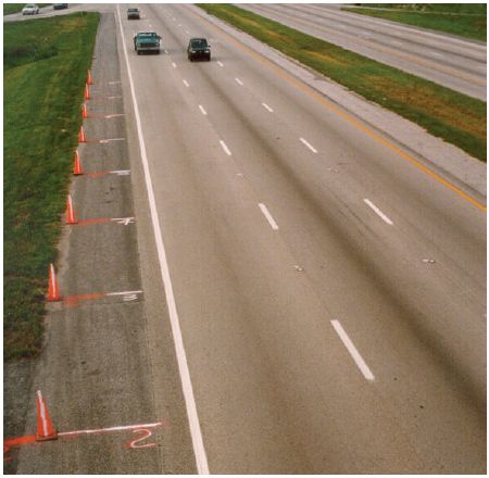
Figure 5-58. Up-lane distance measure aided by traffic cones placed at 25-ft (7.6-m) intervals (temporary markings).
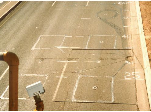
Figure 5-59. Down-lane road surface dimensions marked with paint as used for sensor evaluation and performance comparison.
Some VIPs transmit data to the controller through a serial interface and make the data protocol available to the user. Others require interface or driver software to be purchased or written by the user agency so that their central computer system or controller can interpret the serial data. VIPs also provide data that emulate inductive loop outputs, i.e., optically isolated transitions, so that the VIP data appear to the controller as if they originated from inductive loops. Hence, the controller treats these VIP data in the same manner as inductive-loop data and the same traffic management software can be utilized.
Figures 5-60 and 5-61 contain examples of detection zones drawn for the Autoscope 2004 VIP on the I-5 Freeway in Orange County, CA, as part of the evaluation of a mobile surveillance and wireless communications system.(34) On the mainline (Figure 5-60), vehicle count sensors were connected by AND logical operators to reduce false counts caused by image projection from vehicles into more than one lane. This problem was caused by the relatively low 30-ft (9-m) camera height and side-viewing geometry. Speed sensors (the long rectangular detection zones), presence sensors, and demand sensors were created to demonstrate the different options available for vehicle detection.
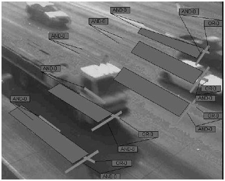
Figure 5-60. Mainline count and speed detection zones for an Autoscope 2004 VIP using a side-mounted camera. Count sensors are represented by the lines perpendicular to traffic flow; speed sensors by the long, rectangular box.
The detection zones on the ramp (Figure 5-61) consisted of demand and count sensors. Sometimes detection zones were placed parallel to the traffic flow direction, and other times sensors were configured in the shape of an × to increase vehicle detection probability. Depending on whether projection of tall vehicle images from one lane into another or occlusion was the more severe problem at a particular site, the × sensors were connected with AND or OR logical operators respectively. OR logic was also applied to increase the probability of vehicle detection by the VIP and the consequent change of signal from red to green. In this application, the primary goal was to prevent vehicles from being trapped at a red signal, rather than concern about a potential increase in false calls.(34)
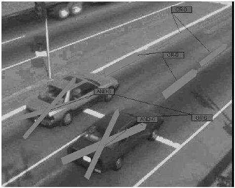
Figure 5-61. Ramp demand zones (× configuration) for an Autoscope 2004 VIP with a side-mounted camera. The zones beyond the stop line record vehicle passage.
Figure 5-62 illustrates the viewing perspective in detection zones created on roadway surfaces, far from low-mounted cameras. The detection zones now enclose a smaller percentage of the pixels in the field of view, decreasing the probability of a detection. In addition, occlusion and projection of tall vehicle images from one lane into another are more prevalent because of the relative size of the detection zone.(34)
Figure 5-63 displays the image and data provided by the Traficon VIP2 traffic data detector, designed for collection of traffic flow data on freeways and arterials.(35) The configuration and data acquisition software operate in a personal computer architecture using RS-232 or RS-485 serial interfaces to the VIP. Data are output to a controller through eight optically isolated semiconductors. The data provided for each lane and the three selectable length-based vehicle classes are volume, speed, gap times, and headway. In addition, the VIP gives the occupancy and density for each lane.
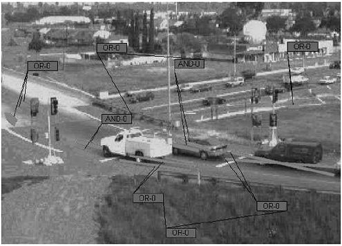
Figure 5-62. Ramp detection zone placement for an Autoscope 2004 VIP when the camera is neither close to the monitored roadway nor at a sufficient height.
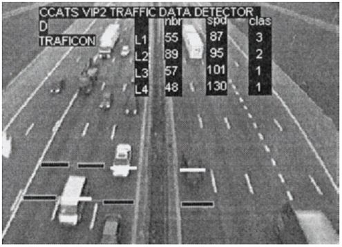
Figure 5-63. Image and data displays for Traficon VIP2 traffic data detector (Source: CCATS® VIP2 Specification. VDS, Inc., San Diego, CA. 1997).
The two types of microwave radars exploited for traffic management are CW Doppler and FMCW presence-detecting sensors. CW Doppler radar sensors detect vehicles traveling at speeds greater than 3 to 5 mi/h (4.8 to 8.0 km/h), but cannot detect stopped vehicles. CW Doppler sensors do not require programming to operate. Most do have jumpers or switches, however, that convey the direction of traffic flow, i.e., approaching or departing, to the sensor. This feature enables some models to detect traffic moving in the wrong direction, such as wrong-way traffic on an entry or exit ramp or on a reversible lane. Presence and passage of moving vehicles are provided from optically isolated semiconductor or relay outputs. Speed is supplied through a serial interface, which usually requires a software driver to be written by the user agency. Some CW Doppler radars allow the detection pattern to be expanded or contracted to cover the area of interest. The antenna design provides the proper beamwidth for measuring traffic parameters over single or multiple lanes, depending on the sensor application, when the sensor is mounted at the recommended height.
Forward- and side-looking radar sensors form elliptical footprints on the road surface. Figure 5-64 defines the footprint and the parameters for a forwardlooking sensor. When the 3-dB antenna beamwidths are available from the manufacturer, the along-lane and cross-lane footprint dimensions can be estimated as(16)
| (5-1) |
| (5-2) |
| where | |
| da, dc =along-lane and cross-lane sensor footprint diameter, respectively | |
| h = R cos θ=sensor mounting height | |
| R =slant range from sensor aperture to center of ground footprint | |
| R sin θ =distance along roadway measured from projection of sensor aperture onto the roadway directly under the aperture to the center of the ground footprint | |
| θa =along-lane two-way 3-dB antenna beamwidth | |
| θc =cross-lane two-way 3-dB antenna beamwidth | |
| θ =angle of incidence of the sensor measured from nadir (downward-looking direction). |
The footprint dimension equations assume that range binning is not used to increase the resolution of the footprint along the major axis. The range bin concept is depicted in Figure 2-59.
Figure 5-64. Microwave sensor detection area for upstream and downstream viewing.
The Whelen TDN-30 narrow beam CW Doppler microwave sensor is mounted centered over the lane of interest (within ± 1.5 ft (0.5 m)) with its bottom surface parallel to the roadway (within ± 5 degrees). With this orientation, the angle of incidence of the antenna with respect to the road surface is 45 deg. The antenna is located inside the sensor housing. The along-lane and cross-lane dimensions of the detection zone are established by the mounting height, as shown in Table 5-22.(36)
| Mounting height | Along-lane beam diametera | Cross-lane beam diametera | |||
|---|---|---|---|---|---|
| (ft) | (m) | (ft) | (m) | (ft) | (m) |
| 15 | 4.6 | 4.2 | 1.3 | 2.9 | 0.9 |
| 20 | 6.1 | 5.6 | 1.7 | 3.9 | 1.2 |
| 25 | 7.6 | 7.0 | 2.1 | 4.9 | 1.5 |
| 30 | 9.1 | 8.4 | 2.6 | 5.9 | 1.8 |
| a Calculated using Equations 5-1 and 5-2 and approximate antenna 3-dB beamwidths of 8 deg for each direction. |
In addition to a jumper for selecting travel direction, the TDN-30 has jumpers that specify the RS-232 data transmission rate (1200 or 2400 baud), transmission mode (modem or free running serial data), operating mode (freeway management, incident detection, or speed and direction detection), dwell count utilized with the incident detection mode, and optically isolated closure time used in the speed and direction detection mode. The freeway management mode permits vehicle speed and count data to be collected. The incident detection mode allows selection of an incident speed threshold and dwell count threshold. If the speed is below the speed threshold, the dwell count is increased by one. If consecutive vehicles, equal in number to the dwell count threshold, are detected below the speed threshold, then a normally open contact is pulsed to indicate the detection of an incident. However, if a vehicle is detected with a speed greater than the speed threshold, the dwell counter is reset.
Once an incident is detected, the sensor begins to measure vehicle speeds to determine if the incident has cleared. An automatic incident cleared speed threshold is calculated equal to the speed threshold plus 25 percent. As before, the dwell counter must increase on consecutive vehicles before a second normally open contact is pulsed, indicating that the incident has cleared. In the speed and direction detection mode, a speed threshold between 5 and 80 mi/h (8 and 129 km/h) is set on thumbwheel switches. As a vehicle is detected, its speed is compared to the threshold. If the speed exceeds the threshold, an optically isolated contact is activated for a user-selectable time of 2, 4, 8, or 16 s.(36)
Some CW Doppler radar manufacturers provide plots of the detection pattern. One such plot is given in Figure 5-65 for the Microwave Sensors TC- 20. The coverage is adjustable by turning a potentiometer clockwise to maximize the pattern size and counterclockwise to minimize it.(37)
Figure 5-65. Approximate detection pattern for Microwave Sensors TC-20 Doppler radar (Source:TC-20 installation instructions. Microwave Sensors, Ann Arbor, MI).
The RTMS presence-detecting microwave sensor combines FMCW and Doppler operation. In its side-fired configuration, it is a multilane sensor capable of detecting stopped or moving vehicles in up to eight lanes. The traffic flow parameters provided per lane are volume, occupancy, speed, and classification based on user-specified vehicle length. In its forward-looking mode, the sensor’s detection zones form a speed trap and measure speed and length of vehicles in a single lane. The speed and length measurements can each be placed in up to seven bins when the sensor is operated in the forward-looking mode. The sensor adds a Doppler speed measurement (maximum error = 2 percent) for speeds exceeding 10 mi/h (16 km/h) in forward-looking operation.
Optically isolated contacts in the RTMS provide presence indication in each detection zone similarly to that of inductive-loop detectors. Thus, the sensor is compatible with controllers that are configured to accept inductive-loop data. Flow rate, occupancy, speed, and classification are available through RS-232 and RS-485 serial interfaces at rates up to 115,200 Baud or through a TCP/IP interface option. Real-time vehicle speed and length are also available for specialized applications, e.g., speed and red light enforcement or excessive speed warning systems.
RTMS setup and calibration are performed using a personal computer and manufacturer-supplied software through an RS-232, RS-485, or TCP/IP interface located on the sensor.(38) The setup wizard can automatically determine the optimum calibration of the RTMS, including operating mode, required number of detection zones and locations, and verify correct operation of the sensor as shown on the setup utility image in Figure 5-66.
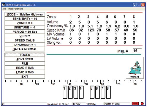
Figure 5-66. RTMS microwave sensor detection zone setup and calibration screen (Image courtesy of EIS Electronic Integrated Systems Inc., Toronto, Canada).
During setup, the lower portion of the figure displays every vehicle within the radar’s field-of-view at that moment as a dark rectangular blip at its corresponding range. A detection zone location is defined by surrounding the blip with a rectangular outline box, which is moved with the arrow keys on the keyboard. A detection zone can include one or more lanes. After a zone is defined, its corresponding optically isolated output contact pair closes every time a vehicle is detected. Once all zones are defined, a manual vehicle count is made and compared with the RTMS count to calculate the accuracy of the setup configuration. If the accuracy is not adequate, the detection zones are adjusted and the manual and RTMS count comparison is repeated.
Early users of the RTMS have remarked about the time needed to accurately aim the radar and calibrate the multiple detection zones when the sensor is in a side-looking configuration to view five or more lanes of traffic. Others have not voiced this concern. Newer versions of the setup software claim to alleviate this issue. Nevertheless, once the viewing angle has been set, sensor performance generally falls within the manufacturer’s specifications.
The single detection zone Accuwave 150LX presence-detecting microwave radar by Naztec also is software programmable from a personal computer using the RS-232 interface on the sensor. Figure 5-67 displays the basic and advanced parameters that can be adjusted.
Figure 5-67. Accuwave 150LX microwave sensor interface and setup options screen (Source: Accuwave 150LX Instruction Manual. Naztec, Inc., Sugar Land, TX).
Basic parameters are cycle time (longest expected intersection cycle time), sensitivity (smaller numbers require a larger signal for a detection), presence timeout (elapsed number of minutes while in a continuous detect state before sensor recycles), detect delay time (elapsed time after sensor detects a vehicle until the sensor becomes active again), and delay inhibit (elapsed time after a vehicle detection before the detect delay time is used again). Advance parameters are sensor identification (address to differentiate a sensor from others on the same communications line), response time (application dependent—intersection applications with slow moving and stationary vehicles require longer response times, hysteresis (low, medium, high), and a fine tuning parameter called profile.(39)
After all entries are made, the download button on the toolbar is pressed to write the parameters into nonvolatile memory in the sensor. The 150LX provides vehicle presence through an optically isolated semiconductor output. The detection area of the 150LX along the road is shown in Figure 5-68.
Figure 5-68. Accuwave 150LX microwave sensor road surface detection area (Source: Accuwave 150LX Instruction Manual. Naztec, Inc., Sugar Land, TX).
Laser radar sensors operate in the near infrared spectrum by transmitting beams that fully scan one or two lanes to provide presence, count, speed, and classification data. Figure 5-69 illustrates the mounting configuration and beam geometry for the Autosense II sensor.(40) The first beam normally has an incidence angle of 10 deg and the second beam an incidence angle of 0 deg. The specified incidence angles are obtained by mounting the sensor with a 5-deg forward tilt, although other mounting configurations can be accommodated. The operating temperature range is from –40 °F to +158 °F (–40 °C to +70 °C) plus sun loading. A 30-minute warmup time is needed at –40 °F (–40 °C).
Figure 5-69. Autosense II laser radar mounting (Source: Autosense II User’s Manual and System Specification. Schwartz Electro-Optics, Inc, Orlando, FL, now OSI Laserscan, 1998).
Autosense II communicates over the factory default RS-422 interface at 57.6 kbaud, 8 data bits, 1 stop bit, and no parity. An optional RS-232 full-duplex serial interface is available. Other outputs include a logic-level vehicle detect line and a solid-state relay (optional). The manufacturer recommends that the data cable be made of low-capacitance polyethylene (such as Belden 9807) as the cable capacitance, which should not exceed 2500 pF, limits the maximum cable length for reliable RS-232 operation.
The Autosense configuration software is executed on a 486 or Pentium personal computer. The data frame format provides frame synchronization, frame start, message, and checksum information. The software menu provides the option of saving all of the data to an ASCII text file. The file name field permits the data to be redirected to another drive. After the software is configured, a power-on message can be accessed to show self-test results, firmware version number, and the measured range to the road for each sample in both beams. A test data output command is available to verify the range and intensity data for each sample in both beams.
Classification is performed by using software that categorizes the profiles of different vehicles. For each vehicle passing through the Autosense II field of view, the sensor outputs five messages based on the location of the vehicle. These messages are as follows:
As the vehicle passes through the first laser beam, the sensor detects the vehicle, assigns a vehicle identification number and outputs Message 1 to the computer. When the front bumper of the vehicle passes the second laser beam, the sensor outputs left edge position, right edge position, and vehicle speed to the computer as Message 2. This message is used to estimate the position of the vehicle. When the rear bumper clears the first laser beam, the left edge position and right edge positions are transmitted from the sensor to the computer as Message 3. As the vehicle continues forward, its rear bumper passes through the second laser beam. Message 4 is transmitted at this time to indicate the end of the vehicle. The Autosense II compiles data accumulated for the vehicle, generates a classification code, a confidence level for the classification estimate, and transmits these data to the computer as Message 5.
Passive infrared sensors contain fixed field of view optics. Some offer a variety of focal length lenses to suit various applications and mounting distances from the detection area of interest. Presence and passage are provided from optically isolated semiconductors or relays. Multiple detection zone passive infrared sensors that measure speed contain a serial interface, which usually requires a software driver to be written by the user agency.
Manufacturers typically provide footprint dimensions for passage infrared sensors as illustrated in Table 5-23.(41) The mounting height h and the range R from the sensor to the center of the ground detection area define the incidence angle θ, as was shown in Figure 5-64. Multiple detection zone passive infrared sensors provide tables that give the dimensions of each zone as a function of mounting height and the distance between the edges of the detection zones and the base of the mounting structure.
The field of view of most ultrasonic pulsed sensors illuminates one traffic lane when they are mounted at the recommended height and pointed directly downward. The one exception is the two-lane Lane King model manufactured by Novax.
Figure 5-70 shows the overhead mounting configuration for the Microwave Sensors TC-30C ultrasonic sensor. The range of the TC-30C is adjusted so that it detects objects at least 2 to 3 ft (0.61 to 0.91 m) above the road surface, e.g., tops of vehicles. The detection gate established by this adjustment differentiates between pulses reflected from the road surface and those reflected from vehicles.
| Mounting height h | Range R | Incidence angle θ | Ground distance d | Footprint width w | Footprint length l |
|---|---|---|---|---|---|
15 ft |
21 ft, 3 in | 45 deg | 15 ft | 2 ft, 8 in | 2 ft, 6 in |
15 ft |
25 ft, 0 in | 53 deg | 20 ft | 3 ft, 1 in | 3 ft, 6 in |
15 ft |
29 ft, 2 in | 59 deg | 25 ft | 3 ft, 8 in | 4 ft, 9 in |
15 ft |
33 ft, 6 in | 63 deg | 30 ft | 4 ft, 3 in | 6 ft, 3 in |
20 ft |
40 ft, 4 in | 60 deg | 35 ft | 5 ft, 1 in | 7 ft, 3 in |
20 ft |
44 ft, 9 in | 63 deg | 40 ft | 5 ft, 7 in | 8 ft, 5 in |
20 ft |
49 ft, 3 in | 66 deg | 45 ft | 6 ft. 2 in | 10 ft, 2 in |
20 ft |
53 ft, 10 in | 68 deg | 50 ft | 6 ft, 9 in | 12 ft, 3 in |
| 1 ft = 0.3 m |
| h = mounting height, d = ground distance between center of the detection area and the base of the sensor mounting structure, R = range from sensor aperture to center of detection area, w = ground footprint width, l = ground footprint length. θ is not selected independently, but is determined from the h and R values through cos θ = h/R. (From: Eltec Instruments, Model 842 Presence Sensor Data Sheet, Daytona Beach, FL.) |
When mounted horizontally, ultrasonic sensors view the side of any vehicles that pass by. In this configuration, the range is adjusted so that the detection zone extends approximately half way through the lane.(42)
Presence and passage are provided from optically isolated semiconductors or relays. Ultrasonic sensors that measure speed contain a serial interface, which usually requires a software driver to be written by the user agency.
The guidelines for installing single-lane and multiple-lane passive acoustic sensor models are described below.
The SmartSonic sensor receives acoustic energy through one beam pointed at the center of the monitored lane. The sensor is aimed by sighting along the tube that serves as part of the mounting hardware.(43) The installation geometry is illustrated in Figure 5-71. The sensor contains an integrated selftest on startup and online, real-time fault monitoring. Optional solar power and spread spectrum wireless transmission link are available to transmit sensor data to a controller. The line of sight range of the wireless link depends on the transmitted power level and bit error rate. Minimum range is 800 ft (244 m) and maximum range is at least 4,800 ft (1,463 m).
Figure 5-70. TC-30C ultrasonic sensor overhead mounting pattern (Source: Microwave Sensors, TC-30C installation instructions, Ann Arbor, MI).
Figure 5-71. SmartSonic acoustic sensor installation geometry (Source: IRD, Inc., Smartsonic Acoustic Vehicle Detection System Specifications) Saskatoon, Saskatchewan. 1996.
The SmartSonic detects vehicle presence through an optically isolated semiconductor. A serial interface on the controller card installed with the sensor provides volume, lane occupancy, speed, vehicle classification (cars, light trucks, heavy trucks and buses), and sensor status messages.
The SAS-1 is designed to monitor up to five lanes when mounted in a sidelooking configuration. Detection zones are created with Windows-based software supplied with the sensor.(44) These zones are equivalent in size to a 6-ft (1.8-m) inductive-loop in the direction of traffic flow and are userselectable in size in the cross-road direction. The software allows monitoring of acoustical signatures and output data as displayed in Figure 5-72. Output data include volume, lane occupancy, and average vehicle speed over a serial interface, which may require interface software to a controller or central computer to be written by the user agency.
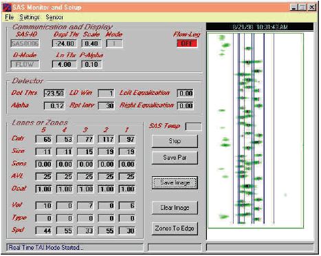
Figure 5-72. SAS-1 acoustic sensor data display (Source: SmarTek Systems, Inc., SAS-1 Specifications, Woodbridge, VA).
The ground footprint dimensions for sensors that utilize combinations of different technologies, such as passive infrared and CW Doppler microwave radar, are specified for each sensor as shown in Table 5-24 and Figure 5-73. In this example, the manufacturer recommends mounting the sensor above the center of the monitored lane facing approaching traffic with the top surface of the unit horizontal or parallel to the road surface if an incline is present.(45) The infrared presence zone is activated as soon as the front of a vehicle enters this portion of the footprint and remains activated until the vehicle leaves. The switching output of the dynamic infrared zone remains activated as long as there is movement detected in this area. The radar measures high to medium speed vehicles and is used by the infrared sensor for speed calibration. Data are output through a serial interface that usually requires driver software to be written by the user agency.
| Mounting height (m) | 5 | 6 | 7 | 8 |
|---|---|---|---|---|
| Doppler radar footprint length (m) | 9.0 | 10.5 | 12.5 | 14.0 |
| Doppler radar footprint width (m) | 2.2 | 2.6 | 3.0 | 3.5 |
| Passive infrared footprint length (m) | 4.0 | 4.5 | 5.2 | 6.0 |
| Passive infrared footprint width (m) | 0.8 | 1.0 | 1.2 | 1.5 |
| 1 m = 3.28 ft |
| (From: ASIM Technologies, Ltd., DT 281 data sheet, Uznach, Switzerland.) |
Figure 5-73. ASIM DT 281 dual technology passive infrared and CW Doppler microwave sensor ground footprints. (Source: ASIM Technologies, Ltd., DT 281 data sheet, Uznach, Switzerland.)
Previous | Table of Contents | Next
FHWA-HRT-06-139 |

