Safety Evaluation of Intersection Conflict Warning Systems

Chapter 4. Methodology

The EB methodology for observational before–after studies was used for the evaluation. This methodology was considered rigorous in that it accounted for RTM using a reference group of similar sites without ICWS installation. In the process, SPFs were used for the following reasons:

• They overcome the difficulties of using crash rates in normalizing for volume differences between the before and after periods.
  
  
• They account for time trends.
  
  
• They reduce the level of uncertainty in the estimates of safety effect.
  
  
• They properly account for differences in crash experience and reporting practice in amalgamating data and results from diverse jurisdictions.
  
  
• The methodology also provides a foundation for developing guidelines for estimating the likely safety consequences of a contemplated strategy.

In the EB approach, the change in safety (Δ) for a given crash type at a site is given by figure 2.

Figure 2. Equation. Estimated change in safety.

Where:

λ = Expected number of crashes that would have occurred in the after period without the strategy.
π = Number of reported crashes in the after period.

In estimating λ, the effects of RTM and changes in traffic volume were explicitly accounted for using SPFs, relating crashes of different types to traffic flow and other relevant factors for each jurisdiction based on reference sites. Annual SPF multipliers were calibrated to account for temporal effects on safety (e.g., variation in weather, demography, and crash reporting).

In the EB procedure, the SPF was used to first estimate the number of crashes that would be expected in each year of the before period at locations with traffic volumes and other characteristics similar to the one being analyzed (i.e., reference sites). The sum of these annual SPF estimates (P) was then combined with the count of crashes (x) in the before period at an installation site to obtain an estimate of the expected number of crashes (m) before installation, as shown in figure 3.

Figure 3. Equation. Empirical Bayes estimate of expected crashes.

Where w is estimated from the mean and variance of the SPF estimate, as shown in figure 4.

Figure 4. Equation. Empirical Bayes weight.

Where:

k = Constant for a given model, which is estimated from the SPF calibration process with the use of a maximum likelihood procedure. In that process, a negative binomial distributed error structure is assumed with k being the overdispersion parameter of this distribution.

A factor was then applied to m to account for the length of the after period and differences in traffic volumes between the before and after periods. This factor was the sum of the annual SPF predictions for the after period divided by P, the sum of these predictions for the before period. The result, after applying this factor, was an estimate of λ. The procedure also produced an estimate of the variance of λ.

The estimate of λ was then summed over all installation sites in a group of interest (to obtain λ_sum) and compared with the count of crashes observed during the after period in that group (π_sum). The variance of λ was also summed over all sites in the strategy group.

The index of effectiveness (θ) is estimated in figure 5.

Figure 5. Equation. Index of effectiveness.

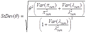
The standard deviation of θ is given in figure 6.

Figure 6. Equation. Standard deviation of index of effectiveness.

The percent change in crashes was calculated as 100(1 - θ); thus, a value of θ = 0.7 with a standard deviation of 0.12 indicates a 30-percent reduction in crashes with a standard deviation of 12 percent.