U.S. Department of Transportation
Federal Highway Administration
1200 New Jersey Avenue, SE
Washington, DC 20590
202-366-4000
Federal Highway Administration Research and Technology
Coordinating, Developing, and Delivering Highway Transportation Innovations
| REPORT |
| This report is an archived publication and may contain dated technical, contact, and link information |
|
| Publication Number: FHWA-HRT-16-036 Date: April 2016 |
Publication Number: FHWA-HRT-16-036 Date: April 2016 |
Since the intersections in Florida and South Carolina likely differ with regard to unobservable variables (e.g., reporting thresholds and driver demographics), matching was done separately for each State. As described in the methodology, binary logistic regression was used to estimate the propensity scores for both States. Since the goal of the binary logit model was to yield matches with good covariate balance, the functional form of the variables in the propensity score models differed between Florida and South Carolina.
The binary logit models estimated the probability that the intersections were CGT intersections (i.e., the propensity score). The models were estimated at the intersection level (all years of data for each intersection). The propensity score model for Florida is shown in table 10, and the model for South Carolina is shown in table 11. For Florida, there were 68 observations, the pseudo R2 was 0.1850, and the log-likelihood was -37.546. For South Carolina, there were 37 observations, the pseudo R2 was 0.3318, and the log-likelihood was -16.911.
| Variable | Coefficient | Standard Error | p-Value |
|---|---|---|---|
| AADTThrough | 0.00009 | 0.00003 | 0.010 |
| AADTIntersecting | 0.00001 | 0.00003 | 0.743 |
| AADTmiss | -1.09534 | 0.99280 | 0.270 |
| THRU_RLT | 0.13667 | 0.67546 | 0.840 |
| INT_RTL | -0.29956 | 0.83036 | 0.718 |
| RAILCROSS | 2.53527 | 1.60811 | 0.115 |
| FRTH_LEG | -0.03758 | 0.95639 | 0.969 |
| CURVE | 0.99022 | 0.70849 | 0.162 |
| SKEW | 0.02244 | 0.02772 | 0.418 |
| THRU_SW | 0.99344 | 0.79216 | 0.210 |
| INT_SW | -0.48141 | 0.66091 | 0.466 |
| Intercept | -3.33964 | 1.56424 | 0.033 |
| Variable | Coefficient | Standard Error | p-Value |
|---|---|---|---|
| LN_AADTThrough | 1.49003 | 1.37409 | 0.278 |
| LN_AADTIntersecting | -0.70140 | 0.41815 | 0.093 |
| THRU_RLT | -0.19744 | 0.92572 | 0.831 |
| INT_RTL | 0.53584 | 1.55880 | 0.731 |
| FRTH_LEG | 1.73509 | 1.14918 | 0.131 |
| CURVE | -0.93645 | 1.36229 | 0.492 |
| Through_Shoulder | -0.24410 | 1.50289 | 0.871 |
| Intercept | -10.5416 | 13.05849 | 0.420 |
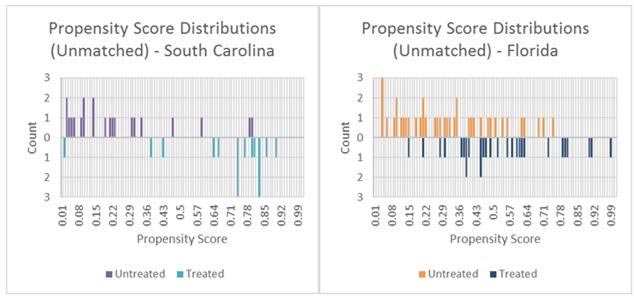
The distributions of the estimated propensity scores for Florida and South Carolina (by intersection type) are shown in figure 17. The box plot of distributions of propensity scores for the unmatched groups show that the ranges of values were similar for Florida and dissimilar for South Carolina. Since the sample size for both States was small, the amount of overlap in the propensity score distributions between CGT and comparison intersections was not large enough to obtain covariate balance using NN matching. When NN matching was used, there were fewer than 10 total intersections from both States combined that matched well based strictly on the estimated propensity scores.

Figure 17. Chart. Plots of estimated propensity scores by State and treatment status.
Since NN matching did not yield the desired covariate balance without a significant reduction in sample size, Mahalanobis matching was implemented. For the Mahalanobis matching using the Florida data, the propensity score, through and intersecting road traffic volumes, through and intersecting road posted speed limits, and intersecting road shoulder width were included as covariates. For Mahalanobis matching using the South Carolina data, the natural log of through and intersecting road traffic volumes, through and intersecting road posted speed limits, and through and intersecting road lane and shoulder widths were included as covariates. Replacement was allowed. No CGT intersection was dropped from the dataset. The majority of comparison intersections were not duplicated for replacement. (Eight intersections were used more than once: seven in Florida and one in South Carolina.)
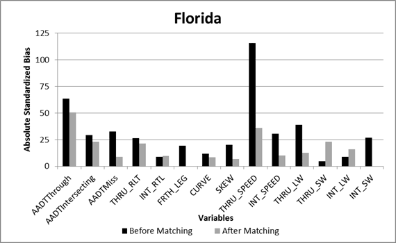
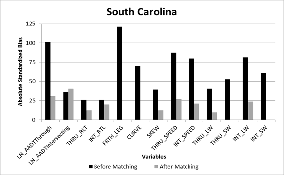
The matching results for both States indicated no significant differences for the majority of the covariates based on the standardized bias. Plots of the absolute standardized bias for each of the covariates are shown for Florida and South Carolina in figure 18 and figure 19, respectively. For Florida, the variables with significant bias (greater than 25 percent) remaining after matching included the through road traffic volumes and posted speeds. For South Carolina, the variables with significant bias remaining after matching included the natural log of through and intersecting road traffic volumes, as well as the through road posted speeds. The Mahalanobis matching was effective at removing the bias in all of the other observed covariates. The variables with significant bias remaining were included in each of the CMF models (added as predictor variables) to account for the differences in the CGT and comparison intersections. By adding the variables with significant remaining bias to the regression model as a predictor variable, the regression model adjusts for the remaining differences in the data for the treated and untreated intersections.

Figure 18. Graph. Absolute standardized bias for covariates in Florida data.

Figure 19. Graph. Absolute standardized bias for covariates in South Carolina data.
Since there were still a number of covariates that were not balanced based on the standardized bias measures, genetic matching was also implemented to improve the matching. K-S tests were then done using the entire sample (both states combined) to help determine the level of covariate balance (for both matching methods and the unmatched data). The results of the tests are shown in table 12.
| Matching Scheme | AADTThrough | AADTIntersecting | AADTMiss | THRU_SPEED | INT_SPEED | INT_LW | INT_SW |
|---|---|---|---|---|---|---|---|
| Unmatched | < 0.0001 | 0.009 | 0.237 | < 0.0001 | 0.032 | 0.077 | 0.097 |
| Mahalanobis matching | < 0.0001 | 0.04 | 0.713 | < 0.0001 | 0.06 | 0.617 | 0.577 |
| Genetic matching | 0.081 | 0.083 | 0.104 | 0.073 | 0.05 | 0.801 | 0.098 |
| Matching scheme | IntNumLane | THRU_LW | THRU_SW | ThruNumLane | FRTH_LEG | CURVE | DEFLECTION |
| Unmatched | 0.265 | 0.001 | 0.133 | < 0.0001 | 0.003 | 0.676 | 0.007 |
| Mahalanobis matching | 0.052 | 0.053 | 0.051 | < 0.0001 | 0.126 | 1 | 0.036 |
| Genetic matching | 0.259 | 0.078 | 0.627 | < 0.0001 | 0.02 | 0.955 | 0.133 |
| Bold = Statistically significant difference (i.e., p-Value ≤ 0.05). | |||||||
As shown in table 12, the K-S tests indicate that the following variables were all significantly different at the 95-percent confidence level using Mahalanobis matching:
The following variables were all marginally different when using Mahalanobis matching:
When using genetic matching, the covariate balance was improved over the Mahalanobis matching. The results of the genetic matching indicate that the only variables that were significantly different between the two groups were INT_SPEED, TruNumLane, and FRTH_LEG.