• Air Toxics
• CMAQ
• Conformity
• It All Adds Up

• Laws and Regulations
• Policy and Guidance
• Research and Analysis
• Training

FHWA and EPA National Near-Road Study - Detroit

13 Appendix - Black carbon measurements

13.1 Digital Aethalometer

Black carbon (BC) was measured continuously at each station using dual-wavelength rackmount Aethalometers (Magee Scientific, Inc.), which is displayed in Figure 60. This report focuses on the results from the main station monitors that were operated for approximately one year.

The Aethalometer continuously measures BC at five minute intervals by pulling air through a small spot on the sample filter and detecting incremental changes in light attenuation at a specific wavelength. Once the sample spot is loaded to a certain limit, the instrument automatically pauses, rotates the filter tape through to a new clean spot, and begins sampling again; this translates to a ten minute gap in the data approximately twice per day in the data set. The main wavelength of light used to detect BC is 880 nm, in the red region of the visible spectrum. In addition, this instrument also detects light attenuation at 370 nm and is a qualitative indicator of additional particulate organics which may absorb light at near-ultraviolet wavelengths.

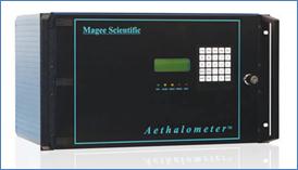
Figure 60 Image of a rackmount Aethalometer (Image source: mageesci.com)

Black carbon values are calculated by the below equation,

BC = ∆ATN *A/ SG* Q*∆t (1)

where, BC is the concentration of black carbon in the sample (units of ng/m^-3), ∆ATN is the change in optical attenuation due to light absorbing particles accumulating on a filter, A is the spot area of filter, Q is the flow rate of air through filter, ∆t is the change in time, SG is specific attenuation cross-section for the aerosol black carbon deposit on this filter (16.6 m²/g). SG is an empirical value that was defined by the manufacturer as the ratio of the mass of elemental carbon (measured using a thermal-optical process) and the detected light absorption of the same sample on a filter.

13.2 . Data Review and Validation

13.2.1 Data time synchronization and screening

BC data was automatically logged by two methods during the Detroit monitoring period - external logging its full set of data fields (17 columns of data) at five minute intervals to a rack-mounted computer, which was downloaded approximately quarterly during the study, and directly logging only the BC concentration estimated from the instrument's analog output to the station database. The analog data was used during the course of the monitoring study to observe the instrument's performance, however the digital data logged to an external rack-mounted computer was used as the primary data for analysis, per manufacturer's recommendations.

NOTE: Sections 14.1 and 14.2 discuss the data processing steps used to analyze the BC data. This discussion was first documented in the Las Vegas Final Report. The steps described were used to post-process the BC data collected during the Detroit study. Figures 57 thru 62 show BC data collected during the Las Vegas study.

Section 14.3 and Section 14.4 which includes Tables 21 thru 23 and Figure 63 report BC data collected during the Detroit study.

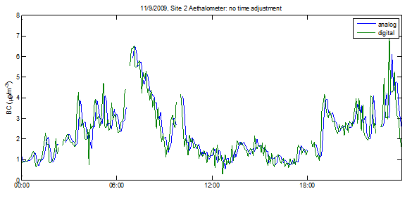
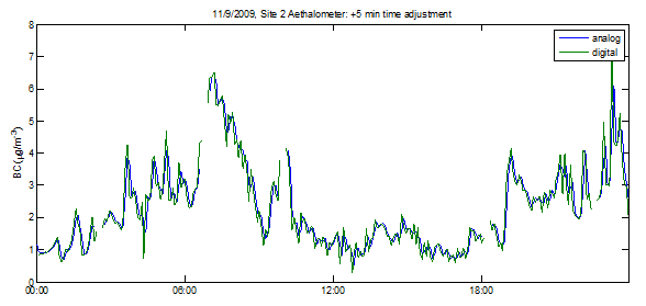
As the digital data timestamp was based on the instrument's internal clock, the first step of data review was to apply any necessary time corrections to the digital data to match it to the station clock. Comparison of analog to digital data streams, as well as viewing the instrument's internal clock, revealed time shifts ranging from 5 min to over 24 hr were needed to precisely overlay the data sets for each station. Each instrument's data was reviewed for time periods throughout the year to ensure that the internal instrument clock did not drift to the point that further time correction was needed. Based on the review, the instrument clocks did not appear to drift by more than 5 min within a one year time period. An example of the time adjustment is shown in Figure 61.

The top image (Figure 61) is prior to time alignment; the bottom image is after the digital data timestamp was adjusted to match the station clock. The breaks in the data indicate time periods when an internal filter change occurred.

Figure 61 Time alignment of analog (blue) and digital (green) data sets.

An additional screen step for the digital BC data was flagging of any data with erroneous light attenuation values (<0 or >60), which affected <1% of the data. Finally, the data are checked for a known logging error that occurs rarely - when a filter change time period spans midnight, the digital timestamp is off by 24 hrs.

13.2.2 Occurrence of negatives

With BC calculated based upon a 5-minute incremental change in light attenuation through a filter, there are time instances when the BC concentrations are generally so low that the accumulation of particles on the filter are not sufficient to override any noise in the measurement (signal to noise ratio), thus the change in attenuation (∆ATN) may read below zero and a negative BC is reported. Since the change in light attenuation is based upon the previous time period, the following time period may then report an overly positive ∆ATN and a higher BC value than reality. The manufacturer recommends that, when negatives occur in the data, one should average the data up to a time increment at which negatives no longer occur. An evaluation of the station 2 BC data is shown in Figure 62, below. In the original 5-minute time series, negatives occur in 2.6% of the data. After averaging up to an hourly time basis, negatives occur in <0.1% of the data. Based upon this evaluation, all data presented in this report are at an hourly time basis and the few, if any, hours of BC data per site that remained negative after averaging were removed from the data set.

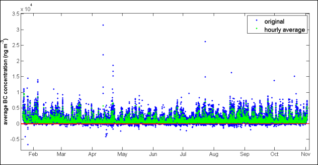
Figure 62 Assessment for negatives occurring in the original data (blue) and hourly averaged data (green) for station 2 during the Las Vegas, NV near-road monitoring study.

13.2.3 Evaluation of filter loading effect

Aethalometers are in widespread use by academic groups and governments to perform continuous monitoring of black carbon in diverse environments. Several research studies have documented that BC values reported by Aethalometers or similar filter-based BC instrumentation may be affected by a filter loading artifact. For example, measured high concentrations of BC in a subway and found that BC values were under predicted as function of filter loading. ²⁰ However, a recent study by measured ambient air quality in India and found that no filter loading effect was detectable in that environment.²¹ The explanation for these differing results likely lies in the optical properties of the particles being measured relative to the samples used for original calibrations by the manufacturer. Since this effect is unpredictable, we did several different analyses to determine whether the artifact existed for the Las Vegas data set and held a meeting to discuss whether or not to apply a correction algorithm.

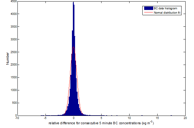
At a mid-way point through the study, an analysis was performed similar to that laid out by looking whether incremental changes (BC at time t+1 minus BC at time t) in BC values revealed a negative bias associated with incremental filter loading.²¹ As shown in Figure 63, below, the histogram of the ∆BC_t+1-t revealed no positive or negative bias and it appeared no significant filter loading effect was detectable, at that time.

Figure 63 Histogram of differences in consecutive BC concentrations (∆BC_t+1-t) calculated at station 1 over data collected during January through April, 2009. The red line is a normal distribution fitted to the data.

At the conclusion of data collection, another analysis approach was employed to determine whether a filter-loading effect was apparent - the attenuation binning method. BC data points collected over a one year period were aggregated into attenuation bins of unit value (0-1, 1-2, 2-3…up to 44-45). A plot of BC data box plots versus attenuation is shown below in Figure 64. Eliminating the tail end values, where fewest BC data points were collected, a modest negative relationship between BC and ATN is visible (Figure 65). Estimating a k-value from this relationship and applying the filter loading correction, it can be seen that BC values at low ATN values would be relatively unchanged while BC values at high ATN values would be increased slightly (Figure 66).²⁰ Overall, this analysis estimated that the filter-loading artifact algorithm would modify concentrations by approximately 0 to +25% depending on the filter loading state.

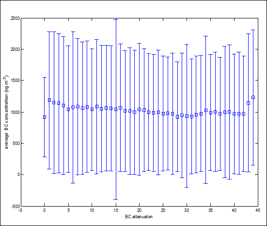
Figure 64 Box and whisker plots of approximately 12 months of 5-minute BC measurements at station 2 aggregated by attenuation bin in one-unit intervals.

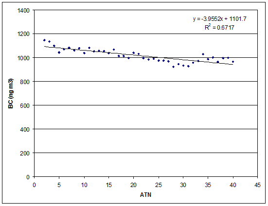
Figure 65 Median BC values of approximately 12 months of 5-minute BC measurements at station 2 aggregated by attenuation bin in one-unit intervals. A linear fit is applied to the data.

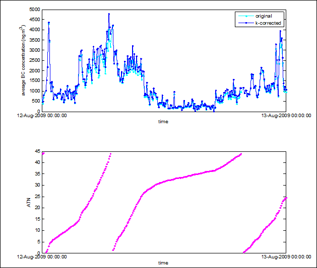
Figure 66 Example of filter-loading corrected versus original data (top) and filter loading attenuation (bottom). At low ATN values, original and k-corrected lines show little difference, while k-corrected BC values are higher than the original at higher ATN values.

One significant concern with applying the k-value correction estimated from the above analyses to the data is that this process essentially assumes that the aerosol optical properties were fixed throughout the measurement period, when in reality the aerosol optical properties likely varied by time of day, day of week, and time of year. Given that a significant amount of data is required to detect the relationship between BC and ATN in an environment with significant ambient fluctuations in concentration, trying to estimate k-values at shorter time increments increases the uncertainty of deriving a reliable value. As the analysis revealed that k-value corrections were relatively minor and given concerns about applying this algorithm without consideration of likely variable aerosol optical properties, it was decided to leave the original data as is for the purposes of this report.

13.3 Data Analysis -- Black carbon measurements

BC data were analyzed using a combination of programs, including MATLAB version R2009b, Microsoft Excel 2007, and JMP 8. The data analysis included calculating summary statistics of data for each site for all wind conditions and for winds only from the South (+/- 60 degrees from perpendicular), estimating concentration gradients for winds from the West, and observing concentrations as a function of wind direction for all winds. The results of these analyses follow in Section 14.4.

13.4 Results and Discussion -- Black carbon measurements

Black carbon data was collected over a one year period at four near-road locations along I-96 in Detroit, Michigan. Hourly concentrations were calculated from the raw five-minute data for each station, covering the time period of the official sampling program - September 29, 2010 to June 15, 2011. The completeness of the data per station is reported in Table 21, which ranged from 97% to 98% per station.

Table 21. Completeness of hourly BC data at each site

Summaries of the annual BC averages and confidence intervals at each site are presented in Table 22 and shown in Figure 67. The data show that, on an average basis with winds from all directions, the BC annual average at 10 m from the highway is significantly higher than at further distances from the road. In addition, BC average values at 100 m in the predominant downwind direction (South of the highway) are significantly higher than at 100 m in the opposite direction, as well as higher than at 300 m on the downwind side of the road. Station 1 BC is approximately 65%, 115%, and 41% higher than Station 2 (100 m downwind), Station 3 (300 m downwind), and Station 4 (100 m upwind) sites, respectively.

Table 22. BC averages for all data (09/29/2010-06/15/2011)

BC hourly values were also isolated for time periods with winds from the west, designated as 180 ± 60 degrees. On the downwind side of the road, BC values at Station 1 are significantly higher than all other stations. Figure 39 and Figure 40 show the mean BC concentrations by site from all wind directions and winds from road, respectively. Station 1 BC is approximately 83%, 167%, and 137% higher than Station 2 (100 m downwind), Station 3 (300 m downwind), and Station 4 (100 m upwind) sites, respectively.

Table 23. BC averages, wind from the West (09/29/2010-06/20/2011)

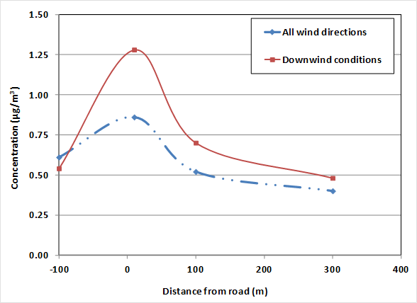
Figure 67 Average black carbon concentrations as a function of distance from the road for all data and during time periods with wind from the South (120-240 degrees).