• Air Toxics
• CMAQ
• Conformity
• It All Adds Up

• Laws and Regulations
• Policy and Guidance
• Research and Analysis
• Training

FHWA and EPA National Near-Road Study Las Vegas

5 Analytical Instruments and Methods

5.1 Data Logging and Time Synchronization

All continuous analyzer data were recorded using an Ecotech 9400TP data logger. These loggers were programmed to record continuous data (averages) at 5-minute intervals. Moreover, these data loggers were time synchronized to National Institute of Standards and Technology (NIST) time by accessing the NIST internet web site hourly and adjusting the data loggers' internal time clock accordingly.

5.2 WinAQMS and WinCollect Software

Ecotech WinAQMS server software was loaded onto the data loggers to handle communications between the continuous analyzers and the data loggers²³. Ecotech WinCollect software was loaded onto a Windows XP workstation at the EPA Facility in RTP, NC to monitor and determine instrument status and performance, perform remote calibrations, determine data validity and download data from the remote field site to the Near-Road database²⁴. This data was loaded into a SAS database for further quality assurance (QA) and data analysis.

5.3 Traffic Activity

Traffic data (vehicle count, vehicle speed, vehicle length) was obtained from the Nevada Department of Transportation's Freeway and Arterial System of Transportation (FAST). This data was an ASCII text file that was sent electronically to EPA. The traffic count system used by FAST is a radar-based system capable of counting and classifying vehicles by length. Each station is equipped with a 10.525 GHz frequency modulated continuous wave (FMCW) radar detector to continuously monitor vehicle length and speed, which includes volumetric flow over multiple lanes with a detection range up to 200 feet. The system can accommodate 6 classes. This traffic data was compiled approximately every 15 minutes and subsequently every hour to provide up to date information on traffic conditions.

Traffic data collected from FAST included two detector sites, one site monitoring the south bound traffic and the second site monitoring the north bound traffic, refer to Table 10. These monitors are located about 400 meters south of the I-15 site. The monitors detect actual free-flow highway conditions without disturbances from on or off exit ramps.

Table 10. Primary Traffic Detectors for I-15 Monitoring Study.

The traffic data totals are always higher than the bin totals, this may indicate that the radar signal from the detector can not provide an appropriate length for binning but recognizes a vehicle present. The differences observed maybe due to partial occlusion of a smaller vehicle by a larger vehicle or improper mounting of the instruments. This trend is seen at both traffic locations.

To help account for these differences a traffic count based upon video recordings were done for sample hours to help determine if the traffic detectors were bias high or low in respect to traffic counts and fleet mix. Vehicles less than 30 feet of length were considered gasoline light-duty (LD) vehicles while vehicles over 30 feet were considered diesel heavy-duty (HD) engines. This comparison of video data with the data loggers will provide a qualitative comparison since visual counts of the vehicles are subject to some level of human error as well. Refer to Figure 17 for a comparison of selected target hours.

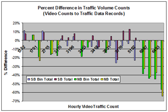
Figure 17. Traffic Count Comparison of Video Data with Traffic Data for I-15.

A quantitative review of the hourly video data with the traffic data logger for Traffic Totals provides a better comparison than the Bin Total for 8 of the 12 hours evaluated for the south-bound (SB) lanes and approximately 9 for the 11 hours for the north-bound (NB) lanes. A further review of the NB data indicates a bias, with the video data providing a significantly lower traffic count than what is recorded with the data loggers. This bias is seen over 90 percent of the time, with percent differences increasing when traffic volume increases. The percent difference ranges from 1 percent to 58 percent, which may result in a two-fold reduction in emissions.

A similar sensitivity analysis was also conducted to compare traffic counts of HD and LD vehicles to determine if a similar bias exists in the traffic data, refer to Figure 18. The average hourly percent difference for HD at times can be rather large approaching 75 percent with an average percent difference for both North and Southbound traffic of about 25 percent. A similar analysis for LD vehicles indicates a bias of the traffic counters over-reporting the NB traffic on an average of 30 percent.

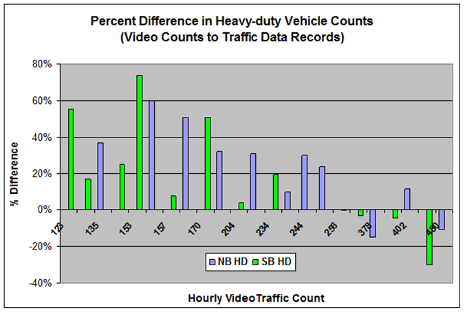
Figure 18. Traffic Count Comparison of Video Data with Traffic Data for HD vehicles on I-15.

A review of the traffic data identifies several periods in time in which the traffic counts and fleet mix do not agree. Some of these anomalies we were able to validate with video evaluations while others show a significant variation with other temporal time periods. Two episodes that were investigated provide an example of why calibrations and evaluations of the traffic data are important.

Episode 1: December 15, 2008 - March 10, 2009

During this period of time the percent HD vehicles for the NB I-15 traffic detector averaged 27%, and then on March 10, 2009 at 6:00 am the HD% changed to 11 percent. The traffic detector from this point thru March 2010 reported an average HD fleet mix of 9 percent. An investigation of this event with the Nevada Regional Transportation Center (RTC) did not identify a cause for this dramatic change in HD percentage.

Episode 2: September 28, 2009 - December 28, 2010

During this period of time the NB traffic volume significantly dropped from an average traffic flow of 3400 vehicles/hour to 1417 vehicles/hour, a 58 percent drop in volume. The NB detector also went off-line on December 28, 2009 and did not come back up until January 22, 2010. A comparison of the video data with the data logger for three hours during this period confirmed the differences; refer to Table 11 with an average percent difference of 61 percent. Investigation of this event with the Nevada RTC did not identify a cause for this dramatic change in traffic volume.

Table 11. Comparison of Video Traffic Count with Traffic Data Logger.

A review of the traffic data log during this period revealed the NB traffic lanes were reduced from 3 lanes to 2 lanes of flow, while a review of traffic video indicates 4 lanes of traffic flow for the NB. Also after December 28, 2009, the NB Detector was switched off with no traffic data being recorded, the monitor was not re-activated until January 22, 2010, at which time it started recording 4 lanes of traffic flow and returns to a normal vehicular flow of 3,900 vehicles/hour. This review of the data indicates the detector was not properly sited to account for all NB lanes during this period. A review of the SB traffic data did not identify any significant abnormal operations.

Traffic speed was recorded by the FAST traffic sensors. Intuitively and based on our own project experiences, as traffic volume increases traffic speed decreases. This is shown explicitly in Figure 19, as traffic volume increases, traffic speed decreases.

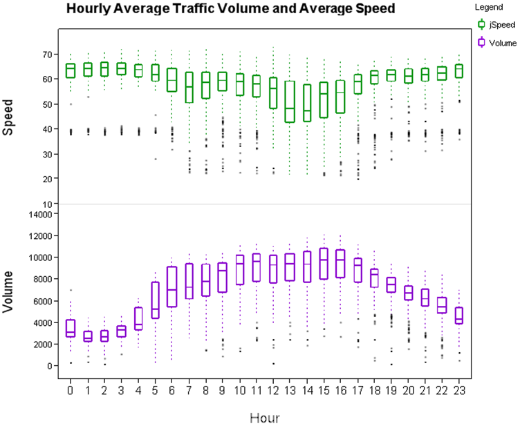
Figure 19. Hourly Average Traffic Volume and Average Speed -- I-15.

5.4 Meteorology

Meteorological monitoring characterized ambient conditions during the day and included measurements for: wind speed, wind direction, ambient temperature, relative humidity, solar radiation, and precipitation. Wind speed and wind direction were characterized by sonic anemometers (R.M. Young Model 81000 Ultrasonic Anemometers). Temperature and relative humidity were characterized by Vaisala HMP45D and Vaisala HMP45A probes, respectively. Solar radiation was measured by a MetOne 394 Pyranometer and precipitation was measured by a rain bucket (Ecotech Rainmaster 1000).

5.5 Continuous Analyzers

5.5.1 Gaseous Pollutants

Gas analyzers (Table 1, Table 12) meeting EPA Federal Reference Method (FRM) or equivalent method criteria collected measurements of CO, NO, NO₂, NO_X, at 100 meters upwind, 20 meter roadside, 100 meters downwind and 300 meters downwind from the freeway. The sample height in all cases was at approximately 3 meters above the ground. Data was logged continuously for 5-minute averaging periods over the course of the study period (Table 13). Multi-point calibrations occurred at the beginning of the study while zero and span checks were run every night over the course of the study period.

5.5.2 Black Carbon

Black carbon (BC) was measured continuously at each station using dual-wavelength rackmount Aethalometers (Table 1, Table 12) at 100 meters upwind, 20-meter roadside, 100 meters downwind and 300 meters downwind from the freeway. The sample height in all cases was at approximately 3 meters above the ground. Data was logged continuously for 5-minute averaging periods over the course of the study period (Table 13).

The Aethalometer continuously measures BC at 5-minute intervals by pulling air through a small spot on the sample filter and detecting incremental changes in light attenuation at a specific wavelength. Once the sample spot is loaded to a certain limit, the instrument automatically pauses, rotates the filter tape through to a new clean spot, and begins sampling again; this translates to a 10-minute gap in the data approximately twice per day in the Las Vegas data set. The main wavelength of light used to detect BC is 880 nm, in the red region of the visible spectrum. In addition, this instrument also detects light attenuation at 370 nm and is a qualitative indicator of additional particulate organics which may absorb light at near-ultraviolet wavelengths.

Black carbon values are calculated by the below equation,

BC = ∆ATN *A/ SG* Q*∆t (1)

where, BC is the concentration of black carbon in the sample (units of ng/m^-3), ∆ATN is the change in optical attenuation due to light absorbing particles accumulating on a filter, A is the spot area of filter, Q is the flow rate of air through filter, ∆t is the change in time, SG is specific attenuation cross-section for the aerosol black carbon deposit on this filter (16.6 m²/g). SG is an empirical value that was defined by the manufacturer as the ratio of the mass of elemental carbon (measured using a thermal-optical process) and the detected light absorption of the same sample on a filter.

BC data was automatically logged by two methods during the Las Vegas monitoring period- internally logging its full set of data fields (17 columns of data) at 5 minute intervals to a compact flash card, which was downloaded approximately quarterly during the study, and directly logging only the BC concentration estimated from the instrument's analog output to the station database. The analog data was used during the course of the monitoring study to observe the instrument's performance, however the digital data logged to the compact flash card was used as the primary data for analysis, per manufacturer's recommendations.

Further details may be found in Appendix 13.

5.5.3 Particulate

Particulate analyzers (Table 1, Table 12) meeting EPA FRM or equivalent method criteria collected measurements of PM-Coarse (particles that have an aerodynamic diameter ranging from 2.5 to 10µm) , PM₁₀ and PM_2.5, at 100 meters upwind, 20 meter roadside, 100 meters downwind and 300 meters downwind from the freeway. Aethalometers and continuous particle counters (Table 12) measured black carbon and particle counts at 100 meters upwind, 20 meter roadside, 100 meters downwind and 300 meters downwind from the freeway. The sample height was at approximately 3 meters above the ground. Data was logged continuously for 5-minute averaging periods over the course of the study period (Table 13).

Continuous PM-Coarse, PM₁₀ and PM_2.5 measurements were collected by four Thermo Electron Tapered Element Oscillating Microbalances (TEOM) Model 1405-DF at a flow rate of 16.7 liters/minute (L/min) (1.0 m3/hour). The data were recorded as 5-minute averages (Table 13).

5.5.4 Integrated Samples - VOC, Carbonyl, Particulate

Specific MSATs of interest for this study included: 1,3-butadiene, benzene, acrolein, formaldehyde and acetaldehyde. MSAT samples were collected using EPA standard methods: 1) TO-15 and 2) TO-11A. The integrated samples were collected on a 1-in12 day ambient air quality monitoring schedule that corresponded to the schedule posted on EPA's website²⁵ and followed by State/local air agencies for ambient air quality monitoring. The EPA PM_2.5 FRM was used for the collection of PM_2.5 integrated samples.

5.5.4.1 EPA Compendium Method TO-15 - Canister - VOC

Collection of canister samples by the TO-15 method calls for the atmosphere to be sampled by the introduction of air into a specially-prepared stainless steel canister. An Entech Model 1816 programmable multi-canister automated sampler was used to accurately regulate the filling of the sample canisters with air. Evacuated SUMMA passivated 6 liter (L) canisters were filled to near ambient pressure. A nominal flow rate of 75 milliliter/minute (mL/min) was maintained over a 1-h sampling period for a total sampled volume of approximately 4.5 L. Evacuated canisters received from the laboratory and ready for sampling were placed on the Entech sampling system by attaching each canister's valve to individual sampling ports. The initial pressure was measured for each canister to insure that every canister falls within an acceptable pressure range (<0.5 psia). Any canisters above the acceptable range were replaced with one that met the initial pressure criteria (0.5 psia). With the canisters attached, each port was leak checked to ensure that fittings had been properly tightened and the samples would not leak prior to and after collection. Sample labels printed with the individual sample codes were affixed to the canister tags for sample identification. The sampler was programmed for the scheduled sampling times and flow rates. Timers and solenoids within the Entech sampler were activated and deactivated allowing sample collection based on the entered sampling program. After the air samples were collected, the canister valves were closed and the canister prepared for shipment to the laboratory for analysis. Sample collection information such as initial and final pressures, initial and final times, canister id number, etc. were either hand recorded on a data collection form for subsequent entry in the electronic data form or entered directly into the electronic data form. Chain-of-custody (COC) sheets were generated and the samples were shipped to the laboratory. Upon receipt at the laboratory, the canister sample label was compared against the datasheet and the COC sheet. Any discrepancies were resolved at that time. The samples were stored until the laboratory analysis of the canisters had been completed.

5.5.4.2 EPA Compendium Method TO-11A - Cartridges - Carbonyl

The EPA Compendium TO-11A DNPH carbonyl method was implemented in Las Vegas for the collection and analysis of air samples for formaldehyde and acetaldehyde. DNPH sampling cartridges are commercially available for this method and were purchased and provided for field sampling. Air samples for carbonyls on DNPH cartridges were collected using an ATEC 8010 automated sampler manufactured by Atmospheric Technology (ATEC). This was the same instrument used for the DNSH cartridge sampling. The instrument is a microprocessor controlled sampler that can be programmed to draw ambient air at a constant rate through various types of sampling cartridges for designated time periods. The sampler consists of two units (channels) each having 10 active sampling ports and one non-active port. Channel 1 (ports 1-10) was used for the DNPH samplers and Channel 2 (ports 11- 20) was used for the DNSH samplers. DNPH samples were collected at a flow rate of 1.00 lpm for a 1-hour time period.

Nine DNPH cartridges were attached to the ATEC's Teflon sampling lines and labeled with the sample collection code. A leak check of each cartridge was performed using the leak check feature of the Atec sampler. This ensured that the cartridges were installed properly. A light blocking sleeve was installed around each cartridge to reduce artifacts due to light sensitivity. The sampler was programmed with the flow, start time and end time for each cartridge channel. During sampling, solenoid valves associated with each cartridge was activated/deactivated based on the programmed sampling schedule. Upon completion of sampling, the cartridges were removed, capped, secured for shipment, and returned via overnight delivery to the EPA RTP facility. Sample collection information such as initial and final flow rates, initial and final times, canister ID number, etc. were either hand recorded on a data collection form for subsequent entry in the electronic data form or entered directly into the electronic data form. COC sheets were generated and the samples shipped to the laboratory. While awaiting shipping, samples were stored in an on-site refrigerator. A cooler with frozen blue ice packs was used to ship the cartridges.

5.5.4.3 Particulate

A BGI PQ 200A PM_2.5 Federal reference method (FRM) sampler was used for the collection of PM_2.5 integrated samples. Cassettes loaded with pre-weighed 46.2 mm Teflon filters were prepared at the EPA RTP facility by EPA contractor staff and shipped to Las Vegas field staff. Filter IDs were linked to unique sample codes generated and printed by data collection spreadsheets. Samples were collected over a 24-hour period beginning at midnight of the sampling day. Flow rates and pressures were recorded by the sampler. At completion, the filter was removed and flow rates and pressures were transcribed onto the data collection spreadsheets. The filter cassettes were removed, packed for shipment, and returned by overnight delivery to EPA RTP.

Table 12. Summary of Measurement Parameters, Sampling Approach, Instruments, and DQI Goals for Project.

2. Accuracy and precision in terms of ultrafine particle concentration is difficult to determine in the field due the lack of particle concentration standards. However, particle counters are routinely verified in the field for accuracy in flow rate. Precision was estimated in this study by collocating UFP samplers prior to use of instruments in the field.

Table 13. Summary of Data Types, Pollutants, Methods and Sample Types and Frequency.

Most analyzers deployed for this study performed well. The ThermoScientific TEOM 1405-DF was upgraded in the field by technical staff from ThermoScientific in late November 2009 and early December 2009. These upgrades improved instrument performance and stability.