
The basic process for calculating emissions involves multiplying VMT by a per-mile emission factor. Thus, accurate VMT forecasts are extremely important for developing emissions estimates in the conformity analysis. This section focuses on the methodologies and approaches used for estimating baseline VMT and forecasting future VMT.
Clearly, any methodology to forecast future VMT requires an accurate estimate of current VMT (and often historic VMT and socio-economic factors as well). Data from the Highway Performance Monitoring System (HPMS) are typically used in small urban and rural areas to estimate VMT for the current year.[4] However, the accuracy of HPMS-based estimates may be limited in small urban and rural areas and for local roadways in particular (as opposed to arterials and other higher functional classifications), given the sparse sample sizes at the county level. As a result, some areas have developed detailed inventories of local road mileage and supplemented the HPMS sample with additional traffic counts, and some have developed detailed traffic monitoring systems in order to develop more accurate estimates of VMT at the county level.
A basic process for estimating VMT using a sample of traffic count data for use in emissions analysis is as follows:[5]
VMT estimates are used together with per mile emissions factors developed using the EPA MOBILE6 model (or EMFAC in California), which in turn, are dependent on speed estimates. As a result, the level of detail in the estimation of VMT will influence the level of detail that can be used in the estimation of speeds, and will ultimately affect the regional emissions estimates.
VMT estimates are typically developed on a daily basis, for multi-hour time periods, or by hour:
1) Average daily VMT - The simplest approach is to develop estimates of average daily VMT by functional roadway classification. Areas with TDF models use modeled volumes by roadway segment. Areas that do not have a TDF model usually rely on HPMS estimates of VMT by functional roadway classification.
2) VMT for different periods of the day - This approach involves developing estimates of VMT for different periods of the day (e.g., AM peak, PM peak, off-peak). This approach is commonly used in areas where there is significant traffic congestion during peak hours. In areas with a TDF model, the model usually can be run to estimate VMT for the morning and evening peak periods, and for total average daily traffic, in which case, the peak periods can be subtracted from the daily total in order to estimate off-peak VMT. Otherwise, average daily traffic estimates can be disaggregated to time periods using locally-developed factors. In areas without a TDF model, average daily traffic is often distributed between peak periods and off-peak periods based on local factors developed from traffic counts.
3) VMT by hour of day - The most detailed breakdown of VMT can be developed by subdividing estimates of daily VMT or VMT by time period to generate hourly VMT. This hourly breakdown is often based on estimates of hourly volumes from a sample of roadways and average roadway speeds each hour. These sample results provide an estimate of VMT for each of 24 hours in the day. This step allows for a more detailed speed analysis in MOBILE6, which allows VMT to be distributed by hour of the day and by speed category or "bin."
In many small urban and rural areas, a simple analysis of average daily traffic will suffice for the regional emissions analysis. However, it is important to recognize cases where a more detailed breakdown is useful to reflect local conditions that could significantly influence emissions.
Moreover, although many areas use annual average daily VMT (based on estimates of annual average daily traffic, or AADT, on roadways), a seasonal adjustment is sometimes applied so the resulting VMT used in the conformity analysis reflects either an average summer or winter weekday, depending on the pollutant of concern (summer for ozone, winter for CO). This seasonal adjustment is most important in areas with large seasonal variations in traffic patterns, and is more often applied in areas that have regional TDF models.
MOBILE6 differs from previous versions of the MOBILE emissions model in that it produces different emission factors for different roadway facility types. The four facility types are:
Using the VMT BY FACILITY command, the user can input the fraction of VMT that occurs on each facility type. The user can run the model assuming 100 percent for a specific facility type in order to develop facility-specific emission factors, or can input a fractional value for each facility in order to develop a composite emissions factor across all road types.
As noted above, MOBILE6 allows users to input VMT information at different levels of detail, depending on the availability of local data. MOBILE6 allows users to specify the distribution of VMT by hour of the day, by speed, and by vehicle type.[6] Using the VMT BY HOUR command in MOBILE6, the user can input the fraction of VMT that occurs at each hour of the day (24 fractional values). The 24 fractions should sum to 1. If this command or other MOBILE6 commands that allow specification of VMT by hour are not used, then MOBILE6 will use national default data for the distribution of VMT by hour.
These methodologies can be used both in areas with or without a TDF model, since TDF models generally do not include road links for local roadways.
For purposes of emissions modeling, note that the assignment of VMT as "local road" VMT may not match with the standard highway classifications of urban local roads and rural local roads. In MOBILE6, local roads are defined as facilities having extremely low average speeds and frequent stops at intersections. They generally represent roads in residential areas and are characterized by having no traffic lights, no more than one lane in each direction, vehicle parking on the street, and traffic control handled via stop/yield signs. MOBILE6 assumes an average speed of 12.9 miles per hour for local roads, which cannot be changed by the user. As a result, roadways that fit within FHWA's "rural local roadways" and "urban local roadways" functional classifications with higher average speeds should be considered arterials/ collectors in MOBILE6. Rural local roadways as defined by FHWA will generally not fit the MOBILE6 definition of local roadways, and many urban local roads will also not fit the definition. Given these differences in definitions, it is important for the analyst to develop an accurate estimate of total VMT in the nonattainment or maintenance area, and to pay special attention to classifying the VMT appropriately into the MOBILE6 road classifications.[7]
VMT Estimation and Forecasting
VMT estimates for local roadways in a particular county are developed by multiplying the HPMS estimates of VMT on collectors in the county by the ratio of local roadway VMT to collector VMT developed using HPMS data at the statewide level (see equation below).

The equation is applied separately for rural local roads, using the proportion of statewide VMT on rural local roads to rural collectors, and for urban local roads, using the proportion of statewide VMT on urban local roads to urban collectors. The estimates of VMT are believed to be more accurate at the statewide level than at the county level, given the limited HPMS sample size at the county level. The same procedure can also be applied using ratios developed at a smaller geographic level than the state (for example, a set of counties within a large state), if sufficient data are available.
This procedure may be used to develop a base year estimate of VMT on local roadways or to forecast VMT on local roadways given a forecast of VMT on collectors.
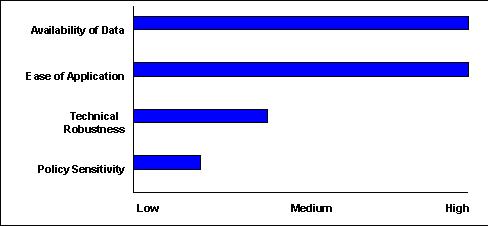
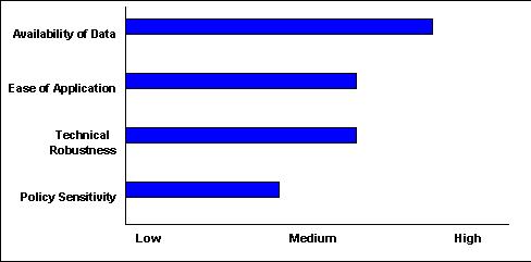
This approach had been used in Kentucky for rural areas and small urban areas (however, this approach is not currently used). In its original approach, the Kentucky Transportation Cabinet (KYTC) examined the statewide ratio of VMT on local roads and collectors, and used the following ratios to predict local road travel in each county: 0.33 (rural local/rural collector), 0.28 (urban local/urban collector in urbanized counties), 0.12 (urban local/urban collector in non-urbanized counties).
Website: http://transportation.ky.gov/Multimodal/Air_Quality.asp
References:
M.L. Barrett, R.C. Graves, D.L. Allen, J.G. Pigman, G. Abu-Lebdeh, L. Aultman-Hall, S.T. Bowling, Analysis of Traffic Growth Rates, University of Kentucky Transportation Center, August 2001.
Bostrom, Rob and Jesse Mayes, "Highway Speed Estimation for MOBILE6 in Kentucky," Kentucky Transportation Cabinet, 2002.
Excel Spreadsheet tables, "2001-2030 VMT Tables," supplied by Jesse Mayes, Kentucky Transportation Cabinet.
This methodology is similar to Method #1, but uses several data points in order to develop a formula relating local road VMT to collector VMT. It relies on several samples of local and collector VMT (e.g., county-level estimates, for various years).
VMT Estimation and Forecasting
An analysis is conducted using available state-level HPMS estimates or county-level samples in order to relate VMT for local roads with VMT for collectors. The analysis can be conducted by testing various equations to describe the relationship between local road and collector road volumes and selecting the best fitting equation. For example, a typical spreadsheet package can test the following:
Simple linear equation[8]: 
Logarithmic equation: 
Exponential equation:nbsp; 
Power equation:nbsp; 
In all cases, a and b are constants that are determined based on the relationship of existing local and collector VMT data.
The formula that is developed from this analysis can then be used to develop an estimate of county-level VMT on local roads given an estimate of county-level VMT on collectors. The formula can be used both for the baseline analysis and projections.
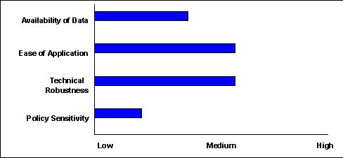
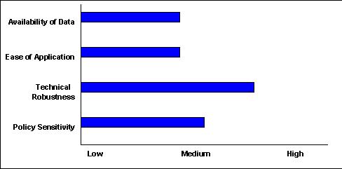
The approach has been used by the Kentucky Transportation Cabinet (KYTC) for small urban and rural areas in order to improve estimates of local road VMT previously developed using Method #1. KYTC used GPS technology to develop accurate mileage data fro local roadways statewide. Reasonably good ADT data at the county level were available from HPMS down to the collector functional class.
Research conducted by the University of Kentucky Transportation Center (see first reference below) found that a simple ratio of local road to collector VMT was inadequate to predict local road VMT. Researchers graphed local ADT against collector ADT to develop the best fitting relationship between these two measures. For Kentucky, they arrived at the following equation:
Local ADT = 3.3439 x (Collector ADT)0.6248
KYTC selected to use this equation rather than a simple ratio since they found that local roads carry much less traffic relative to collectors in locations where collectors have higher VMT. Therefore, if a simple ratio had been used as in method #1, then local road VMT would have been overestimated where collector VMT was relatively high.
Website: http://transportation.ky.gov/Multimodal/Air_Quality.asp
References:
M.L. Barrett, R.C. Graves, D.L. Allen, J.G. Pigman, G. Abu-Lebdeh, L. Aultman-Hall, S.T. Bowling, Analysis of Traffic Growth Rates, University of Kentucky Transportation Center, August 2001.
Bostrom, Rob and Jesse Mayes, "Highway Speed Estimation for MOBILE6 in Kentucky," Kentucky Transportation Cabinet, 2002.
Excel Spreadsheet tables, "2001-2030 VMT Tables," supplied by Jesse Mayes, Kentucky Transportation Cabinet.
Not Applicable (only rated for forecasting methodologies)
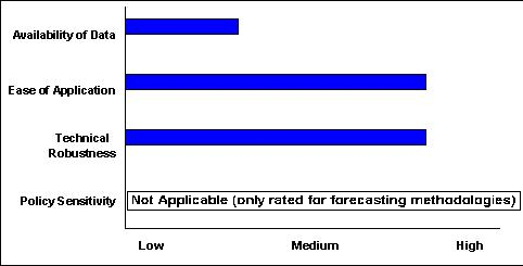
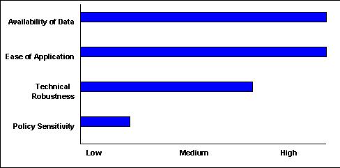
* Note: This method is used solely to develop an estimate of baseline VMT for local roadways, with or without a TDF model. Projections can be made using any of the methods described in Sections 2.4 or 2.5, depending on whether a TDF model is available; a very simple approach is to estimate and apply a growth factor.
VMT Estimation
A detailed inventory of total road mileage on local roadways is required. Traffic counts are conducted in order to develop estimates of average daily traffic (ADT) on a sample of local roadways in the area of interest. The ADT estimates are then applied to the appropriate road links or assumed to apply to other nearby links. Alternatively, an overall average ADT can be applied across all road mileage. VMT is estimated by multiplying ADT by the link length.
North Carolina DOT (NCDOT) applied this methodology in conducting analyses of regional emissions in donut areas outside of MPO boundaries. NCDOT records AADT for all roads in all functional classifications. Since less than 74 percent of local road mileage was covered by actual counts, for local road links without traffic counts, NCDOT assumed 400 ADT. This is the maximum amount of traffic expected on low-volume local roads.[9]
The Rogue Valley MPO in Medford-Ashland (Klamath County), Oregon, used an assumption of 20 ADT on unpaved roads in the base year as part of its conformity analysis for the 2004-2007 Transportation Improvement Program (TIP). The ADT average was developed by the Oregon Department of Transportation's Transportation Planning and Analysis Unit. The MPO assumed a growth rate of 1.2 percent per year for future projections.
References:
North Carolina DOT, Davidson County, and the North Carolina Department of Environment, "Emissions Analysis Report for the Transportation Plan for the Rural Portion of Davidson County." September 27, 2002.
Rogue Valley MPO, "2004-2007 Transportation Improvement Program and
Air Quality Conformity Determination," August 26, 2003.
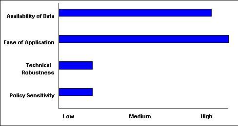
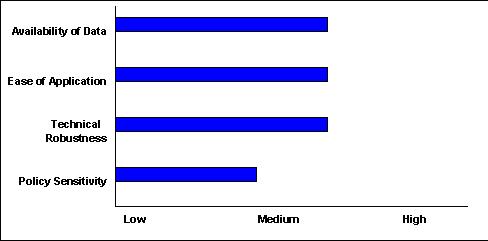
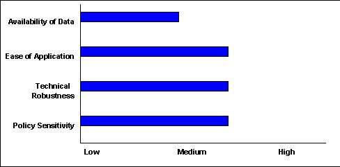
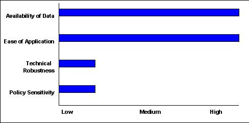
It should be noted that although these methodologies all rate relatively low in terms of policy sensitivity (their ability to respond to changes in highway investments, transit investments, or other policies), separate analyses can be conducted in order to evaluate the effects of new transportation investments, including highway facilities, transit services, park and ride lots, and other transportation control measures. Small urban and rural areas often conduct special analyses of these types of investments to assess the effect to which they might be expected to bring in additional "through" traffic, change the routes that drivers take, or shift drivers from motor vehicles to transit or higher occupancy modes. The effects of these investments on VMT is then added to or subtracted from the totals resulting from the general VMT projection methods.
VMT Projection
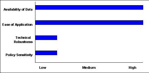
VMT projections are developed by applying an estimated VMT growth rate to a base-year estimate of VMT, developed from traffic counts and data on roadway extent. Regional planners develop the VMT growth rate based on historical information or expectations for future growth using demographic or other projections. Projected VMT is then apportioned to the functional classes in the same ratio as the most recent year of VMT data.
Colorado DOT used this approach in one conformity analysis conducted in Aspen, a rural nonattainment area for PM-10. The VMT forecast was based on a baseline estimate of VMT for 1990 from vehicle counts, projected to future years based on an estimated growth rate of 2 percent per year. This overall growth rate was estimated by City of Aspen planners based on experience with recent trends and anticipated growth patterns.
This approach can also be applied for a particular type of roadway (i.e., local roadways, unpaved roads) when a model does not address the roadway class. For instance, the Rogue Valley MPO in Medford-Ashland (Klamath County), Oregon, assumed a growth rate of 1.2 percent per year for future projections of VMT on unpaved roads as part of its conformity analysis for the 2004-2007 Transportation Improvement Program (TIP).
Website:
http://www.dot.state.co.us/environmental/CulturalResources/AirQuality.asp
References:
Colorado DOT, "Colorado State Implementation Plan for PM-10, Aspen Element." Revised September 22, 1994.
Colorado DOT, "Air Quality Analysis, A Technical Report to the State Highway 82 Entrance to Aspen Environmental Impact Statement," July 7, 1995.
Rogue Valley MPO, "2004-2007 Transportation Improvement Program and
Air Quality Conformity Determination," August 26, 2003.
VMT Projection
VMT projections are developed on a county basis based on the historical trend line (an ordinary least squares linear regression extrapolation of the latest ten years of data). The statistical analysis uses total VMT in order to avoid issues associated with reclassification of VMT over time due to the expansion of urbanized boundaries and other functional class shifts. Projected VMT is then apportioned to the functional classes in the same ratio as the most recent year of VMT data.
The approach has been used by the North Carolina DOT for the donut areas in North Carolina where a metropolitan area's travel demand model includes the metropolitan planning area only and not the balance of the nonattainment or maintenance area.
Web sites:
http://www.ptcog.org/emissions.pdf
References:
North Carolina DOT, Davidson County, and the North Carolina Department of Environment, "Emissions Analysis Report for the Transportation Plan for Rural Portion of Davidson County," September 27, 2002.
VMT Projection
VMT forecasts are developed based on a linear regression for each functional class of roadway. However, in order to use historic data to conduct a linear regression by functional class, adjustments need to be made to correct for minor changes in functional class categories (associated with changes due to system upgrades).
Minor changes are "smoothed" by adjusting the historic annual VMT for a particular functional class in proportion to any subsequent changes made in functional class mileage (do to roadway upgrades). Per the equation below, this is done by multiplying VMT for each year by the ratio of mileage in the functional class in the current year to mileage in the VMT estimate year (for example, if current mileage on urban arterials is 105% of mileage in a historic year, due to system upgrades, VMT on urban arterials in the historic year will be multiplied by 1.05 in order to get an adjusted VMT estimate).
For each roadway functional class, for each historic year:
This effectively adjusts the older VMT for a given functional class to account for roadways that have since been shifted into that functional class. Per the equation below, functional class VMT totals must then be adjusted to ensure that total VMT for each year does not change as a result of these adjustments. The VMT sum for each year is calculated, and the ratio of the original VMT sum to the new VMT sum is multiplied by the adjusted VMT value for each functional class.
For each roadway functional class, for each historic year:

To avoid problems caused by larger discontinuities in historic trends by functional class (for example, due to changes in the definition of a functional classification at a particular time), linear regressions are conducted in a manner so they do not span such discontinuities. In other words, if a major jump takes place in 1990, the regression may disregard all data prior to 1990.
The procedures discussed above may be conducted at the statewide level in order to develop projected growth rates for each functional class that can then be applied at the local level.
Ohio Department of Transportation (DOT) uses TDF models for many small urban areas. Where there is no TDF model, Ohio DOT has used this procedure to forecast VMT. In this case, VMT estimates were only believed to be accurate at the statewide level, not the local level. As a result, the procedures for estimating future VMT growth rates were conducted at the statewide level for all functional classes in order to maintain consistency. The statewide growth rates were then applied to estimates of VMT by functional class for the area being analyzed.
Website: http://www.dot.state.oh.us/urban/index.htm
(See VMT forecasting procedures described under "documents" section:
VMT Projection
Interstate VMT is projected using linear regression based on historic traffic volumes.
Non-Interstate VMT is calculated by multiplying projected population by projected non-Interstate VMT per capita. Projected population can be taken from the MPO or state agency responsible for population projections. Non-Interstate VMT per capita is forecast based on a linear regression using historic estimates of VMT per capita for non-Interstate travel at the county level. This forecast recognizes that the amount of daily travel per person has increased historically and is likely to continue to increase. The resulting estimate of non-Interstate VMT is then apportioned to the functional classes in the same ratio as in the most recent year of data (also see Method #5 below for an alternative methodology for estimating non-interstate VMT).
The approach has been used by the South Carolina Department of Transportation in Cherokee County.
References:
Gardner, John, "Vehicle Miles of Travel Projections and Speed Estimates for Rural Nonattainment and Maintenance Areas," South Carolina Department of Transportation.
VMT Projection
Interstate VMT is projected using data on historic trends, but is assumed to decline somewhat based on limitation in highway capacity or other factors. A corridor-by-corridor analysis is conducted of historic VMT growth in order to develop an initial annual growth rate. An adjusted annual growth rate is then developed for purpose of projections based on professional understanding of the anticipated pace of traffic growth in each corridor.
An estimate of non-Interstate VMT is developed using an approach similar to the one described in methodology #4, which relies on projections of population and per capita VMT. However, in this case, statewide growth in non-Interstate VMT is estimated using statewide VMT data from HPMS and state population estimates. First, a linear regression is developed to predict statewide non-Interstate VMT as a function of population, based on historic data, as follows:

The base year non-Interstate VMT is then subtracted from the future year projection to calculate the projected growth in non-Interstate VMT. This statewide VMT growth is then allocated to the counties based on a combination of county population change and a projected increase in per capita VMT, as described below:
The resulting estimate of county-level non-Interstate VMT is then allocated to each functional class in the same proportion as in the HPMS baseline year.
The approach has been used by the Kentucky Transportation Cabinet (KYTC) in locations where there is not a TDF model.
References:
M.L. Barrett, R.C. Graves, D.L. Allen, J.G. Pigman, G. Abu-Lebdeh, L. Aultman-Hall, S.T. Bowling, Analysis of Traffic Growth Rates, University of Kentucky Transportation Center, August 2001.
VMT Projection
VMT forecasts for each county and functional class are based on traffic data and growth factors that reflect historic correlations between VMT and population and employment for each county and functional class. The growth factor employs a decay function assuming that VMT growth will taper off. Estimates are adjusted to reflect current year HPMS VMT estimates.
The approach has been used by the Pennsylvania Department of Transportation for all areas where there is not a TDF model.
Reference:
Michael Baker, Jr., Inc., "The 2002 Pennsylvania Statewide Inventory, Using MOBILE6, An Explanation of Methodology," November 2003.
Areas that maintain a TDF model generally use the model outputs to estimate VMT. There are a variety of commercially available TDF model software packages in use, including TranPlan, TransCAD, TP+, Viper, MINUTP, EMME/2, and QRS2. Software is often supplemented by custom sub-routines not integrated into the package. The scope of these models also differs - some areas have urban area models, some county-level models, and a few have statewide models (which may not use commercial software) that provide county-level data. At least one State reported using both urban area models (for the MPO area) and a statewide model (for the donut areas outside of MPO and urban model boundaries).
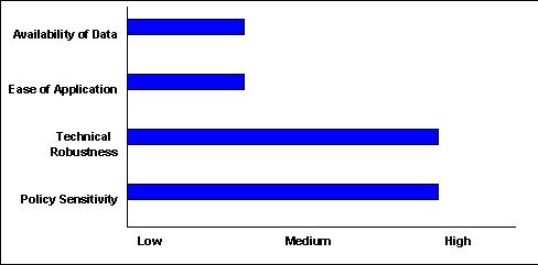
TDF models offer greater sensitivity to changes in transportation investments or policies, compared to most manual calculation procedures. New facilities and improvements to existing facilities can be coded into the network. In estimating future VMT, the TDF model takes into account all of these improvements at once, predicting the most likely distribution of traffic on the future network. In contrast, most off-model calculation procedures cannot consider how all improvements together would affect traffic distribution across the network.
Adjustments to TDF model outputs are often required in order to make the results suitable for conformity analysis. Adjustments to the model outputs generally fall into three categories:
In cases where a TDF model is available, the model itself is generally used to estimate future VMT by functional class. However, some adjustments may be made to the estimates so they can be used for the regional emissions analysis. The adjustments are typically made either to improve the reliability of the estimates or to ensure that the resulting estimates are consistent with estimates from HPMS that were used in developing the emissions budget in the SIP.
Samples of adjustments include:
VMT Estimation
When a travel demand model is used to estimate VMT, those estimates must be checked against HPMS VMT estimates and adjusted if needed. The goal is to ensure, as best possible, that the travel demand model is forecasting VMT consistently with the VMT reported through the HPMS system.
VMT estimates from the TDF model are compared to the VMT estimate from HPMS for each functional class in the base year. Adjustment factors are calculated for each roadway functional class to fit the modeled VMT estimates to the HPMS estimates, as follows:

VMT Projection
VMT projections are made using the TDF model in a standard fashion. The adjustment factors for each functional class developed in the base year comparison are then applied to all forecast years to scale the forecasts.
This adjustment is required under the transportation conformity rule, and always should be applied in areas with TDF models to come up with accurate forecasts. Michigan DOT, for instance, uses adjustment factors to scale the results of the urban area models that it maintains for all small urban areas. In Yuma County, Arizona, VMT figures on local roadways were scaled up since the model local roadway mileage was 136 miles, whereas the actual local roadway mileage was approximately 780 miles.
References:
Michigan DOT, Travel Demand Analysis Section. "Technical Documentation of the Procedures Used to Develop VMT and Speed Estimates for Michigan Non-Attainment Counties Containing a Modeled Urban Area." 1995.
Lima & Associates "Vehicle Particulate Emissions Analysis" prepared for ADOT, and Yuma MPO, May 2002.
VMT Estimation and Projection
Baseline VMT is estimated for each link using a TDF model. Based on professional expertise, knowledge of a given location, or review of travel activity data, selected road links or classifications are subject to a downward adjustment to represent trips traveling a limited distance along the links. The adjustment factor is then applied to future forecasts on those links or functional classes.
The approach has been used in Yuma County, Arizona, where final VMT was adjusted down in rural areas by a certain percentage for local paved roads and by another percentage for local unpaved roads.
Reference: Lima & Associates "Vehicle Particulate Emissions Analysis" prepared for ADOT, and Yuma MPO, May 2002.
VMT Estimation and Projection
An off-model, customized procedure is developed to account for external trip purposes that may represent significant VMT and be sensitive to predictable factors. These may include external-internal trips and external-external (through) trips. Although these trips are typically accounted for in traffic assignment based on traffic counts, this procedure includes a detailed analysis and projection methodology to better predict potential changes in the rate of external trips. For tourist trips, projected population increases in states that supply the largest number of visitors and anticipated growth in service employment can be used to estimate the number of external trips and VMT generated.
The approach has been used by the Maine DOT in its statewide TDF model. The statewide model relies on population demographics, employment, and economic activity in order to forecast VMT. A REMI model[10] was used to establish base year and forecast year population and employment for nine regions in Maine. By using a REMI model for population and employment estimates Maine's statewide TDF model accounted for vehicle travel that may be specifically associated with large transportation investments.
A separate category of external trips was developed for tourist travel into Maine. Maine DOT reviewed population increases in states that supply the largest number of visitors to Maine (Massachusetts, Connecticut, Rhode Island, New York, and New Jersey) and projected growth in service employment in order to come up with an estimated increase in external trips.
Website: http://www.maine.gov/mdot/aqn/
Reference: Maine Department of Transportation (Bureau of Planning), "The 2002 - 2004 STIP Conformity Analysis for Maine's Nonattainment and Maintenance Areas," August 2001.
VMT Estimation and Projection
A scaling factor is developed to scale the annual average daily VMT estimates to reflect a summer or winter season. The scaling factor is developed by dividing average daily traffic in the season of interest by average annual daily traffic (AADT). The data come from traffic surveys conducted at various points in the year.
Pennsylvania DOT (Penn DOT) developed an automated software package called PPSUITE, which takes the daily volumes from its Roadway Management System (RMS) that represent AADT, and seasonally adjusts the volumes to reflect an average weekday in July. The Pennsylvania DOT developed the adjustment factors for each functional class of roadway based on the ratio of weekday July traffic counts to the RMS's data on annual average volumes.
Reference:
Michael Baker, Jr., Inc., "The 2002 Pennsylvania Statewide Inventory, Using MOBILE6, An Explanation of Methodology," November 2003.
Many TDF models only include the higher functional classifications of roadways, not roadway functional classes with low traffic volumes such as local roads. Accounting for future local road links in TDF models is often problematic since the construction of local streets is dependent upon private residential development and is not included in regional transportation plans, and therefore, it is difficult to determine where and how many local roads will be built in future years. Moreover, some areas may not have an accurate inventory of all local roads. However, in order to estimate regional emissions, estimates of VMT on the entire road network are required.
As a result, areas with TDF models typically use off-model procedures to forecast VMT on local roadways. Several methods can be used to estimate VMT for local roads that are not covered by a regional TDF. Some of the methods described earlier in Section 2.3 (i.e., Method 1: Use statewide HPMS data to calculate the proportion of local road VMT to collector VMT; or Method 2: Use county-level HPMS estimates to develop a statistical relationship between local road VMT and collector VMT) can also be applied in areas with TDF models.
The methods described in this section rely on information from the TDF model. The two sample methods are:

VMT Estimation and Projection
VMT on local roads is assumed to be a consistent percentage of modeled VMT. For example, if local road VMT is assumed to be 10% of the modeled VMT, and the model produces an estimate of 100,000 daily vehicle miles, then local road VMT would be estimated as 10,000 vehicle miles, for a regional total of 110,000 vehicle miles. The percentage may be determined based on available data sources, such as HPMS figures for the county or state by functional class.
This methodology was used Medford-Ashland (Klamath County), Oregon, by the Rogue Valley MPO in its air quality conformity determination for the 2004-2007 TIP. The Rogue Valley MPO has a TDF model that estimates average daily VMT within the MPO area but does not include local streets. In this case, VMT on local streets in the MPO area was assumed to be 10 percent of the modeled VMT.
References:
Rogue Valley MPO, "2004-2007 Transportation Improvement Program and
Air Quality Conformity Determination," August 26, 2003.
VMT Estimation
VMT estimates are taken directly from the TDF model for functional roadway classes included in the model. For those classes of roads not included in the model, the VMT estimate is taken directly from HPMS.
VMT Projection
VMT growth rates for non-represented functional classes are assumed to be parallel to those of a functional class that is represented in the model (e.g., local roads are assumed to have the same growth rate as collectors). For example, if the model forecasts that VMT on rural collectors will increase 15% between the base year and the forecast year, then VMT on rural local roads would be assumed to increase by 15%.
The approach has been used by Michigan DOT in the portion of Allegan County that is outside of the area covered by the model used for the MPO area by the Macatawa Area Coordinating Council (MACC).
References:
"Technical Documentation of the Procedures Used to Develop VMT and Speed Estimates for Michigan Non-Attainment Counties Containing a Modeled Urban Area," Travel Demand Analysis Section, Michigan DOT, 1995.
VMT Estimation
Baseline VMT is estimated for each local link in a traffic analysis zone (TAZ), based on the link length (derived using a GIS application) and the number of vehicle trip-ends generated within the TAZ. These two factors may be statistically evaluated against those local roads for which data are available, and a relationship thus developed.
VMT Projection
Future year VMT on local roads is estimated as base year VMT plus additional VMT associated with new development. Since the number of lane miles of new local roads is unknown, the incremental VMT is estimated based on the projected increase in the number of dwelling units in the TAZ and an estimate of daily VMT on local roads per dwelling unit. Local road VMT per dwelling unit is estimated based on a linear regression of historical values from travel surveys.
The approach has been used in Yuma County, Arizona, where local roads in the regional transportation network were not represented in the TransCAD model.
An inventory was performed on all local streets in the region to obtain relevant information, such as their location and surface type. In this case, link VMT for local roads in the base year was calculated using the equation:

The VMT for future off-network links could not be estimated by the foregoing expression, since it is difficult to estimate the future construction of local roads. However, a simple linear regression analysis revealed that a relationship exists between the VMT and the number of dwelling units in a TAZ.
The analysis found that, on average, daily VMT on local roads for a TAZ increased by 1.22 mile for every increase in one dwelling unit. The increase in VMT on local roads for a specific TAZ was thus estimated as 1.22 times the number of dwelling units added to the TAZ between the base year and the future year.
References:
Lima & Associates "Vehicle Particulate Emissions Analysis" prepared for ADOT, and Yuma MPO, May 2002.
In many cases, the geographic area covered by an MPO TDF model is inconsistent with the boundaries of the non-attainment or maintenance area that must be examined for the regional emissions analysis. In cases where the non-attainment or maintenance area is larger than the MPO planning area covered by the TDF model, the total VMT for the entire area is usually estimated through a two part process: 1) the MPO's TDF model is used to estimate VMT in the MPO area (along with any necessary adjustments, as discussed in sections 2.5.1 and 2.5.2), and 2) separate off-model approaches are used to estimate VMT in the portion of the nonattainment or maintenance area outside of the coverage of the TDF model (i.e., the donut area).
A range of off-model approaches can be used to estimate VMT for the donut area. This section identifies three methods that utilize outputs of the TDF model:
In addition, the methods discussed in section 2.4 for forecasting VMT without a TDF model typically can be applied in donut areas.
VMT Estimation
Countywide VMT estimates are based on estimates of Annual Average Daily Traffic (AADT), drawn from the best available data sources. For many areas, the annual HPMS VMT estimates reported to FHWA are the best available data. Some states also collect additional traffic counts and may have better estimates of traffic at the county or MPO level. For local road links without counts, assumptions of AADT can be made. VMT values for the modeled area are subtracted from the county-wide values by functional class to get the base year VMT by functional class for the donut area.
VMT Projection
VMT projections are developed on a county basis based on the historical trend line (e.g., an ordinary least squares linear regression extrapolation of the latest ten years of data). The statistical analysis can use total VMT in order to avoid issues associated with reclassification of VMT by functional class over time due to the expansion of urbanized boundaries and other functional class shifts. Projected VMT is then apportioned to the functional classes in the same ratio as the most recent year of VMT data.
The modeled area VMT forecast is then subtracted from the countywide VMT forecast for each functional class to obtain estimates of the donut area VMT by functional class.
The approach has been used for the donut area of Sheboygan County, Wisconsin, where The Bay-Lake Regional Planning Commission conducts the conformity analysis for the Sheboygan County maintenance area using a regional travel demand model for the area within the MPO boundary, and simpler HPMS-based forecasting methodology for the rural donut portion of the county.
References:
Bay-Lake Regional Planning Commission, Wisconsin DOT, and Wisconsin Department of Natural Resources, Assessment of Conformity of the Year 2025 Sheboygan Area Transportation and the 2004-2007 Sheboygan Metropolitan Planning Area Transportation Improvement Program (TIP) with Respect to the State of Wisconsin Air Quality Implementation Plan, Fall 2003.
VMT Estimation and Projection
An estimate of baseline VMT on high-ADT roads is developed by multiplying ADT on these road links by the link length. The ADT figures come from traffic counts collected along freeways and major arterials. To forecast future VMT, an estimated annual traffic growth rate is applied to the baseline estimate. The traffic growth rate is estimated based on historical data and/or information on factors that may affect future traffic growth.
VMT on low-ADT roads is then estimated using the ratio of VMT on low- to high-ADT roads from the modeled area, as follows:

For example, if low-ADT roads contribute 30% of the VMT of high-ADT roads in the modeled area, VMT on low-ADT roads in the donut area is assumed to be 0.3 times VMT on high-ADT roads in the donut area.
The approach has been used in Medford-Ashland (Klamath County), Oregon, by the Rogue Valley MPO area for the conformity analysis of the 2004-2007 TIP. The Rogue Valley MPO has a TDF model that estimates average daily VMT within the MPO. An "off-model" calculation was conducted for roadways outside the MPO area. VMT on arterials and interstates in non-MPO areas was estimated based on traffic counts and estimated traffic growth rates developed by the Oregon Department of Transportation; VMT on collectors and local roads in non-MPO areas was estimated based on the same ratio of VMT on these roads to arterials and interstates as inside the MPO area.
References:
Rogue Valley MPO, "2004-2007 Transportation Improvement Program and
Air Quality Conformity Determination," August 26, 2003.
VMT Estimation and Projection
Base year and future year estimates of VMT for the MPO planning area are calculated using the MPO's TDF model. Base year and future year estimates of countywide VMT are developed using the statewide TDF model (Since statewide models do not include all roadway links, expansion factors are developed for each functional class by taking the HPMS county-level VMT estimate and dividing by the modeled VMT estimate for each functional class; the expansion factors by functional class are then applied to all future year VMT forecasts).
Estimates of VMT from the MPO's TDF model are then subtracted from the total countywide VMT estimates from the statewide TDF model to determine VMT in the portion of the county not covered by the MPO's TDF model.
Local roads are not incorporated into statewide models, so county-level HPMS figures are used for the base year. VMT growth for those local roads is assumed to parallel growth on collectors, and future year VMT figures are calculated accordingly.
The approach has been used by Michigan DOT for donut areas outside of MPO boundaries in small urban areas, such as Allegan County. Michigan DOT maintains a statewide TDF model, which is used in these analyses.
References:
Michigan DOT, Travel Demand Analysis Section. "Technical Documentation of the Procedures Used to Develop VMT and Speed Estimates for Michigan Non-Attainment Counties Containing a Modeled Urban Area." 1995.
[4] The HPMS provides data that reflects the extent, condition, performance, use, and operating characteristics of the nation's highways. For more information on background, scope, major uses of the HPMS, and reporting requirements, consult FHWA's HPMS Field Manual at http://www.fhwa.dot.gov/policyinformation/hpms/fieldmanual/.
[5] Adapted from Guidance for the Development of Facility Type VMT and Speed Distributions, U.S. EPA, Report Number M6.SPD.004, February 1999.
[6] Methods for estimating VMT by speed bin are discussed in Section 3. Methods for estimating VMT mix by vehicle type are discussed in Section 4.2.
[7] The MOBILE6 emissions model functions differently than MOBILE5, which simply developed emission factors based on average speeds. As a result, methodologies for conformity analysis using MOBILE5 did not need to make this distinction between the different definitions of local roadways, and commonly developed emissions estimates based on average speed by functional roadway classification.
[8] This formula is nearly equivalent to method 1, except that it allows for a certain baseline VMT level on local roads that is independent of the volume on collector roads.
[9] American Association of State Highway and Transportation Officials, A Policy on the Design of Highways and Streets [2001 Greenbook], 2001.
[10] A REMI model (Regional Economic Models, Inc.) is a commonly used economic-forecasting and policy-analysis model;

