• Air Toxics
• CMAQ
• Conformity
• It All Adds Up

• Laws and Regulations
• Maps
• Policy and Guidance
• Research
  • General Practice
  • Air Quality Planning and SIPs
  • Emissions Analysis
  • Land Use
  • Multi-Jurisdictional (Complex) Areas
  • Project Level Conformity
  • Small Urban and Rural Areas
  • Tools & Methodologies
  • Transportation Control Measures
• Resources
• Models & Methodologies
• Training
• Air Quality Newsletter

Sample Methodologies for Regional Emissions Analysis in Small Urban and Rural Areas

4 Other Factors: Sample Techniques to Improve Upon MOBILE Defaults

4.1 Background

The MOBILE6 model (and EMFAC) takes into account a number of factors in estimating emission rates. In addition to vehicle speeds, important factors that influence emission rates include: the mix of vehicles that contribute to VMT, the age distribution of the vehicle fleet, the mix of VMT by type of roadway, and the existence and type and scope of inspection and maintenance (I/M) programs in place.

The MOBILE model contains default values for many of these factors, which may be used for simplicity. However, the MOBILE defaults may not reflect local conditions, and small urban and rural areas may want to identify data and use approaches to improve upon default values. This section describes several approaches to potentially improve upon default values.

4.2 VMT Mix by Vehicle Type

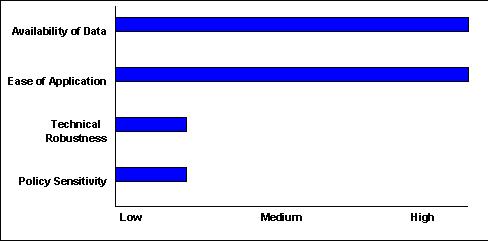
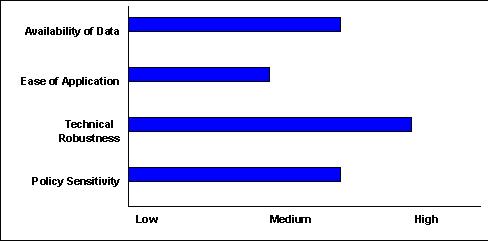
The VMT fleet mix determines how the VMT is assigned to each vehicle type (or class). Emission factors across vehicle classes may vary widely (greater than a factor of 100), so that even small changes in fleet mix have the potential for large changes in emission totals. Some of the small urban and rural areas have identified that getting the vehicle mix properly specified for their region was an important factor in helping their region meet conformity.

MOBILE6 users can enter information on VMT by vehicle class using the VMT FRACTIONS command. MOBILE6 uses 28 vehicle classes. However, for MOBILE6 VMT inputs, the 28 vehicle classes are consolidated into 16 vehicle classes shown in the table below. (The 28 classes are consolidated essentially by combining gasoline and diesel vehicles of a given class). Thus, the user inputs a set of 16 fractional values, representing the fraction of total VMT accumulated by each of the 16 combined vehicle types. The 16 values must sum up to 1.

Note: These class divisions are not likely those used in local vehicle registration systems or in reporting VMT data to the Federal Highway Administration's (FHWA) Highway Performance Monitoring System (HPMS), so care must be taken when relating vehicle types across these data sources.

If no information on VMT mix by vehicle class is entered, model default values are used. The MOBILE6 default values were developed from national-level vehicle registration data by age and class, as reported for July 1, 1996. EPA developed a methodology to convert the July 1, 1996 registration profile into a general registration distribution by age and by vehicle category for the 16 composite vehicle types and up to 28 individual vehicle classes. To forecast future changes, EPA evaluated general sales growth and vehicle scrappage trends for the total light-duty vehicle in-use fleet and the total heavy-duty vehicle in-use fleet, and made minor adjustments, where possible, to reflect some of the differences between vehicle categories.

Estimating VMT Mix by Vehicle Type

Method 1: Use MOBILE6 Model Defaults

Description

The MOBILE model requires estimates of a distribution of registered vehicles by age and vehicle category for current and future years. For MOBILE6 new national level vehicle registration data by age and class were developed for July 1, 1996. EPA developed a methodology to convert the July 1, 1996 registration profile into a general registration distribution by age and by vehicle category for some 16 composite (gasoline and diesel) vehicle types. To project future changes EPA evaluated general sales growth and vehicle scrappage trends for the total light-duty vehicle in-use fleet and the total heavy-duty vehicle in-use fleet, and made minor adjustments, where possible, to reflect some of the differences between vehicle categories.

Method Applicability

This method is most applicable in a nonattainment or maintenance area where it is anticipated that the vehicle fleet mix is similar to the national default. This is most applicable in areas that parallel the national socioeconomic statistics. This assessment should include all on-road vehicles in the area including those outside the nonattainment or maintenance area if a considerable portion of vehicles in the on-road fleet come from outside the area.

Data Sources and Procedures

This approach involves using the national default registration distribution that comes with the MOBILE6 model. A review of the national registration data should be made in order to verify the appropriateness of the national default data. This review could look at the most important class of emissions light-duty vehicles and heavy-heavy duty vehicles. Also, an assessment should be made as to the projected trends in sales growth and scrappage trends to determine if the default trends used in MOBILE6 are appropriate.

Advantages

• Uses a readily available, nationally recognized source of data that requires little effort for the user to apply.
• Use of the national average facilities comparisons to other regions using the national averages for the fleet mix distribution.
• The approach is simple to operationalize.

Limitations

• The area's VMT fleet mix may vary significantly from the national default. Thus, the approach may not provide a valid representation of the actual fleet mix.
• The approach does not include local adjustments for changes in local scrappage or sales rates. Localized shifts in these trends may have substantial impact on emissions.

Example Location

This methodology has been applied in Portneuf Valley, Bannock County, Idaho. It was suspected that the higher proportion of SUVs would be found in this county than the national default. A local vehicle count was conducted in the area, which verified that the national defaults were in the appropriate range for this category.

Resources:

Bannock Planning Organization, "FY2004 Draft Transportation Improvement Program Conformity Determination," August 15, 2003.

Estimating VMT Mix by Vehicle Type

Method 2: Use Available Local Data and Maintain Constant Mix for Future Years

Description

The MOBILE model requires estimates of a distribution of registered vehicles by age and vehicle category for current and future years. In this case, local registration and/or local traffic data are used to characterize the vehicle mix for the 16 composite MOBILE6 vehicle classes (or potentially the full 28 MOBILE6 categories), and this mix is assumed to hold constant over future years.

Method Applicability

This approach is most applicable in areas where there are significant differences in the local vehicle fleet mix relative to the national average vehicle fleet mix, and where changes are not anticipated in the future. It is most applicable where the local traffic and/or registration data can be assembled and are representative of the nonattainment or maintenance area. Both traffic survey and registration data at the local level can be used to estimate vehicle fleet mix. However, if only local registration data are used, adjustments may be needed if a significant portion of on-road motor vehicles come from outside the nonattainment or maintenance area.

Estimating VMT Mix by Vehicle Type

Method 2a: Use Local Vehicle Registration Data

Data Sources and Procedures

This approach involves using local vehicle registration data. This is typically available at the county level, but may be possible to acquire at city or smaller scale from the state motor vehicle registrar office. The fleet mix should be representative of the vehicle mix over the small urban or rural area under question. If the pollutants of concern are ozone precursors then the data should reflect the July 1^st date. For CO, the January 1^st date should be used.

Also, an assessment should be made as to the projected trends in sales growth and scrappage trends to determine if the default trends used in MOBILE6 are appropriate when using this local vehicle registration data for baseline fleet composition. The extent to which the growth and scrappage trends diverge from the baseline is an important factor that will affect estimates of future year emission estimates.

Advantages

• Uses locally specific registration data that is likely more representative of the local area than the national default.
• Requires minimal additional resources, particularly if data is readily available at the county or local level from the State department of motor vehicle registration.
• Recommended by EPA and is generally accepted as a viable approach.

Limitations

• Registration data may include vehicles owned, but not operated in the local area.
• Registration data does not differentiate between seasonal usage differences in vehicles. For example, in some locations, light-duty trucks (LDTs) are operated more frequently in the winter months with the need for better traction in winter driving conditions; conversely light-duty vehicles (LDVs, or passenger cars) are used in summer months when driving conditions are less demanding.
• Does not include local adjustments for changes in local scrappage or sales rates. Localized shifts in these trends may have substantial impact on emissions.

Example Location

This methodology has been applied in a number of counties in Pennsylvania. The distributions were developed for July 1^st and reflect the development of the fleet mix for the group of 16 composite MOBILE6 vehicle types. However, Pennsylvania elected not to use the heavy-duty vehicles registration data as they were limited and because much of Pennsylvania's HHDDV traffic is through traffic. Pennsylvania used the MOBILE6 defaults for HHDDV. This approach was also used in Missoula County, Montana with the same mix in future years.

References:

"The 2002 Pennsylvania Statewide Inventory, Using MOBILE6, An Explanation of Methodology," Michael Baker, Jr., Inc., November 2003.

Estimating VMT Mix by Vehicle Type

Method 2b: Use of Traffic Data for Each Vehicle Class

Data Sources and Procedures

This approach involves using county traffic count data by vehicle class. This requires data collection on a representative set of facilities over the small urban or rural area under question. The data collection requires measuring as many of the 28 MOBILE6 vehicle classes as possible. At a minimum the counts should be able to separate out LDGV, LDGT, and HDDV. If the pollutants of concern are ozone precursors then the data should reflect the July 1^st date. For CO, the January 1^st date should be used.

Also, an assessment should be made as to the projected trends in sales growth and scrappage to determine if the default trends used in MOBILE6 are appropriate when using this county traffic data for baseline fleet composition. The extent to which the growth and scrappage trends diverge from the baseline is an important factor that will affect estimates of future year emission estimates.

Advantages

• Uses county traffic count data, which are more representative of the local area than the national default.
• Requires minimal additional resources, particularly if traffic count data by vehicle class are readily available from the State DOT.

Limitations

• The county traffic count data by vehicle type require a moderate level of increased resources to complete.
• It may be difficult to gather more than a handful of vehicle classification data from the county traffic count data.
• The traffic count data should reflected the climate season of concern; fleet mix may change significantly in some locations.
• The approach does not include local adjustments for changes in local scrappage or sales rates. Localized shifts in these trends may have substantial impact on emissions.

Example Location

This methodology was used in Bannock County, Idaho to verify the percentage of LDGT1 and LDGT2 trucks had been properly developed for their region. The results showed that the national defaults were very similar to the local fleet fractions for LDGT1 and LDGT2 vehicles.

References:

Bannock Planning Organization, "FY2004 Draft Transportation Improvement Program Conformity Determination," August 15, 2003.

Estimating VMT Mix by Vehicle Type

Method 2c: Use of a Combination of Traffic Data and Vehicle Registration Data

Data Sources and Procedures

This approach involves using traffic count data by vehicle class in combination with vehicle registration data. This requires data collection on a representative set of facilities over the small urban or rural area under question and ideally the local vehicle registration. The traffic data collection count requires collecting information on vehicle type by roadway functional class. The vehicle registration data are then used to determine the type of fuel use by vehicle type. The vehicle registration data are typically available at the county level, but may be possible to acquire at city or smaller scale from the state motor vehicle registration office. The product of the registration data and traffic count are used to determine the MOBILE6 fleet mix over the small urban or rural area under question. If the pollutants of concern are ozone precursors then the data should reflect the July 1^st date. For CO, the January 1^st date should be used.

Also, an assessment should be made as to the projected trends in sales growth and scrappage to determine if the default trends used in MOBILE6 are appropriate when using this baseline fleet composition. The extent to which the growth and scrappage trends diverge from the baseline is an important factor that will affect estimates of future year emission estimates.

Advantages

• Uses traffic count data, which are likely more representative of the local area than the national default.
• Uses local registration data, which is likely more representative of the local area than the national default.
• Offers an approach to develop an estimate for the full 28 MOBILE6 vehicle classification categories.
• Appealing in estimating fleet mix in the near future as the alternative fueled and new technology (hybrid vehicles - gasoline/electric and diesel/electric) begin to enter the fleet.

Limitations

• The traffic count data by functional class require a moderate level of increased resources to complete.
• The need to acquire the vehicle registration data and compute the product with the traffic count data entails a modest amount of additional resources.
• The traffic count data should reflect the climate season of concern; fleet mix may change significantly in some locations.
• The approach does not include local adjustments for changes in local scrappage or sales rates. Localized shifts in these trends may have substantial impact on emissions

Example Location

This methodology was used in Cheshire County, New Hampshire. VMT mix was estimated by using a combination of vehicle registration data and traffic count data were collected by roadway function class. County registration data was used to estimate fuel use (gasoline, diesel) by vehicle type and the cross product used to estimate the sixteen MOBILE6 vehicle mix categories. Development of a local fleet mix was identified as an important factor in helping the region meet conformity.

References:

New Hampshire Department of Transportation, "Procedure to Determine VMT Percentages by Vehicle Type in New Hampshire", August 2, 2002.

Estimating VMT Mix by Vehicle Type

Method 3: Use Available Local Data for Base Year Fleet Mix and Iteratively Adjust To Reflect Expected Changes in Mix

Description

The MOBILE model requires estimates of a distribution of registered vehicles by age and vehicle category for current and future years. In this case, local registration and/or local traffic data are used to characterize the vehicle mix for the 16 composite MOBILE6 vehicle classes (or potentially the full 28 MOBILE6 categories). The estimates are then iteratively adjusted for each analysis year in proportion to changes assumed in the MOBILE default values.

Method Applicability

This approach is most applicable in areas where important differences are known relative to the national average vehicle fleet mix used in MOBILE6. It is applicable where the local traffic data in conjunction with vehicle type from the HPMS reporting system can be assembled and is representative of the nonattainment or maintenance area under study. Ideally, traffic survey count information classified by vehicle type at the local level can be used to estimate on-road vehicle fleet mix for the MOBILE6 model. Caution is advised in mapping the HPMS vehicle type information to the MOBILE6 model as the two classification schemes are distinctly different.

Data Sources and Procedures

This approach involves using local traffic count data by vehicle class. This requires data collection on a representative set of facilities over the small urban or rural area under question. The data collection requires using historical HPMS data for the six or more vehicle classification counts and then translating to the 16 MOBILE6 composite vehicle classes. These vehicle classification counts from HPMS are used in conjunction with the default MOBILE6 vehicle mix by iteratively adjusting the distributions so that the final fleet mix reflect the change in vehicle mix for each year. At a minimum the vehicle classification counts should be able to separate out LDGV, LDGT and HDDV. If the pollutants of concern are ozone precursors then the data should reflect the July 1^st date. For CO, the January 1^st date should be used.

Also, an assessment should be made as to the projected trends in sales growth and scrappage trends to determine if the default trends used in MOBILE6 for future years are appropriate when using this local traffic data for baseline fleet composition.

Advantages

• Uses traffic data classification counts, which are likely more representative of the area than the national default.
• Uses only a modest additional resource requirement by using historical HPMS data; particularly if representative traffic data vehicle classification counts are readily available from the State DOT.

Limitations

• The traffic count data by vehicle type require a moderate level of additional resources to complete.
• It may be difficult to gather more than a handful of vehicle classification data from the HPMS traffic classification count data.
• The traffic count data should reflect the climate season of concern; fleet mix may change significantly in some locations.
• The approach does not include local adjustments for changes in local scrappage or sales rates projected for future years. Localized shifts in these trends may have substantial impact on emissions.

Example Location

This methodology was used across North Carolina for six urban and six rural road types. It was used primarily for adjusting the vehicle classification mix to reflect the change in fleet mix for higher light-duty truck fraction than the national average using recent historical HPMS data.

Reference:

Phone conversation with Behshad Norowzi, North Carolina DOT, bnorowzi@dot.state.nc.us), February 17, 2004.

4.3 Vehicle Age Distribution

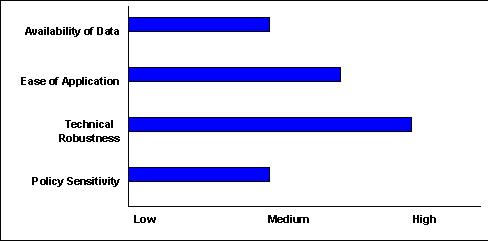
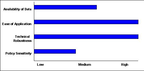
The vehicle age distribution determines the fraction of vehicles operating within each emissions control requirement standard and the deterioration of the emission control technology. Emission rates vary widely between new and older vehicles. Thus, even small changes in fleet age, particularly for older vehicles, may result in large changes in emission totals.

The MOBILE6 model requires estimates of a distribution of registered vehicles by age and vehicle category for current and future years. MOBILE6 default values were developed using national level vehicle registration data by age and class for July 1, 1996. EPA developed a methodology to convert the July 1, 1996 registration profile into a general registration distribution by age and by vehicle category for some 6 composite (gasoline and diesel) vehicle types plus motorcycles (see Table below). To project future changes, EPA evaluated general sales growth and vehicle scrappage trends for the total light-duty vehicle in-use fleet and the total heavy-duty vehicle in-use fleet, and made minor adjustments, where possible, to reflect some of the differences between vehicle categories.

MOBILE6 U.S. Vehicle Fleet Distribution of Registration Fractions by age as of July 1

Note: age 1 = 75% of age 1 as predicted by the curve fit analysis to reflect a July 1 population of age 1 vehicle.

Estimating Vehicle age Distribution

Method 1: Use MOBILE6 Model Defaults

Description

The MOBILE model requires estimates of a distribution of registered vehicles by age and vehicle category for current and future years. This approach uses the national default registration distribution in MOBILE6.

Method Applicability

This method is most applicable in a nonattainment or maintenance area where it is believed that the vehicle fleet age is similar to the national default. This is most likely the case in areas that parallel national socioeconomic statistics. This assessment should include all on-road vehicles in the area including those outside the nonattainment or maintenance area if a considerable portion of vehicles in the on-road fleet come from outside the area.

Data Sources and Procedures

This approach involves using the national default registration distribution that comes with the MOBILE6 model. A review of the national registration data should be made in order to verify the appropriateness of the national default data. This review could look at the most important classes of vehicles: light-duty gas vehicles and heavy-duty diesel vehicles.

Also, an assessment should be made as to the projected trends in sales growth and scrappage trends to determine if the default trends used in MOBILE6 are appropriate. The extent to which the growth and scrappage trends diverge from the national default in the future is an important factor that will affect estimates of future emissions.

Advantages

• Uses a readily available, nationally recognized source of data that requires little effort for the user to apply.
• Use of the national average facilities comparisons to other regions using the national averages for the vehicle age distribution.

Limitations

• Area may have a VMT age distribution that varies significantly from the national default. Thus, the approach may not provide a valid representation of the actual fleet age distribution.
• Sensitivity tests conducted by EPA^[15] found that only a 20% age shift to older vehicles can increase emissions for hydrocarbons and CO by as much as 50% depending on the calendar year of evaluation and up to 40% for NO_x.
• Approach does not include local adjustments for changes in local scrappage or sales rates. Localized shifts in these trends may have substantial impact on emissions.
• Use of national defaults may have important implications on policy decisions if vehicle registration fees are tied to age of vehicle (i.e., as done in many counties to help reduce emissions a policy could be made to increase license fees as the vehicle ages to encourage people to use newer low-emitting vehicles)

Example Location

This methodology has been applied in Portneuf Valley, Bannock County, Idaho. However, efforts were underway to obtain a VIN decoder that would enable them to use a county specific fleet age distribution because of concerns about using the national default values for this small urban area of Pocatello and Chubbuck.

References:

Bannock Planning Organization, "FY2004 Draft Transportation Improvement Program Conformity Determination," August 15, 2003.

Estimating Vehicle age Distribution

Method 2: Use Local Vehicle Registration Data for In-Use Fleet

Description

The MOBILE model requires estimates of a distribution of registered vehicles by age and vehicle category for current and future years. This approach uses local vehicle registration data to develop these inputs.

Method Applicability

This approach is most applicable in areas where there are significant differences in the local vehicle fleet age distribution relative to the national average. It is most applicable where the local registration data can be assembled and are representative of the nonattainment or maintenance area. Ideally, registration data at the local level can be used to estimate vehicle age distribution. However, adjustments may be needed if a significant portion of on-road motor vehicles is from outside the nonattainment area.

Data Sources and Procedures

This approach involves using local vehicle registration data. This is typically available at the county level, but may also be applied using statewide data from the state motor vehicle registration office. The fleet age should be representative of the vehicle fleet over the small urban or rural area under question. If the pollutants of concern are ozone precursors, then the data should reflect the July 1^st date. For CO, the January 1^st date should be used.

Also, an assessment should be made as to the projected trends in sales growth and scrappage trends to determine if the default trends used in MOBILE6 are appropriate when using this local vehicle registration data for baseline age distribution. The extent to which the growth and scrappage trends diverge from the baseline is an important factor that will affect estimates of future year emission estimates.

Advantages

• Uses locally specific registration data, which is likely more representative of the local area than the national default.
• Requires minimal additional resources, particularly if data is readily available at the county or local level from the State department of motor vehicle registration.
• Recommended by EPA and generally is encouraged as a preferred approach over the national default approach.

Limitations

• May include vehicles owned, but not operated in the local area.
• Registration data does not differentiate between seasonal usage differences in vehicles. For example, in some locations LDGT are operated more frequently in the winter months with the need for better traction in winter driving conditions. Conversely, more LDGV are used in summer months when driving conditions are less demanding.
• Does not include local adjustments for changes in local scrappage or sales rates. Localized shifts in these trends may have substantial impact on emissions.

Example Location

The basic methodology has been applied in several locations, including Cheshire County, NH and in Missoula County, MT.

In Berks County in Pennsylvania, the Pennsylvania Department of Transportation used the same approach, except for heavy-duty vehicles, where the distribution was estimated using the internal MOBILE6 age distributions, since much of Pennsylvania's heavy-duty vehicle traffic is through traffic and therefore not registered in the state.

The Bay Lake Regional Planning Commission in Wisconsin used the same approaches but distributions were only made at the highest level for the three major vehicle classes of LDGT, LDGT and HDDV. Also, data were only applied using state registration distributions.

For small urban and rural areas in North Carolina, the North Carolina Department of Transportation developed age distributions based on registration data for the eight vehicle types for those portions of the state outside the state's three major urban areas.

References:

Bay-Lake Regional Planning Commission, "Assessment of Conformity of the Year 2025 Sheboygan Area Transportation Plan and the 2004-2007 Sheboygan Metropolitan Planning Area Transportation Improvement Program with Respect to the State of Wisconsin Air Quality Implementation Plan," 2003.

New Hampshire Department of Transportation, "Procedure to Determine VMT Percentages by Vehicle Type in New Hampshire", August 2, 2002.

Montana Department of Environmental Quality, Vehicle Fractions by Functional Roadway Classifications, February 25, 2004.

Pennsylvania Department of Environmental Protection, "The 2002 Pennsylvania Statewide Inventory Using MOBILE6, An Explanation of Methodology," Prepared by Michael Baker, Jr., Inc. November 2003.

4.4 Percent of VMT on Freeway Ramps

In the MOBILE6 model, there are four sets of driving cycles that are modeled separately, representing different types of functional classes of roadways:

• Freeway (excluding ramps)
• Arterial/collector
• Local roadway
• Freeway ramp

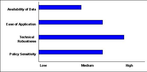
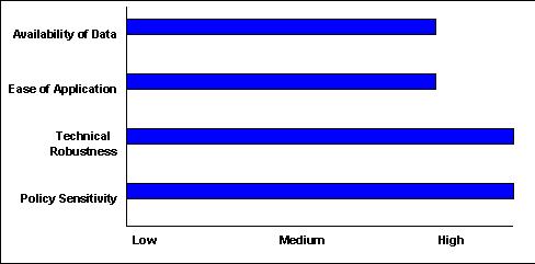
The fraction of vehicle miles traveled (VMT) by highway functional system (also called "roadway type" or "facility type") varies from area to area and can have a significant effect on overall emissions from highway sources. For SIP-related highway vehicle emission inventory development in moderate and above non-attainment areas, EPA expects states to develop and use their own specific estimates of VMT by highway functional system. Each driving cycle may be run separately, with analysis results combined outside of the MOBILE6 model, or the user may use the ability of MOBILE6 to combine the results into a single composite emission rate.

It is important for transportation agencies to understand what the MOBILE roadway classifications represent since each driving cycle set implies different assumptions about vehicle activity and different emission estimates in MOBILE6. These classifications may not always match with definitions used by transportation agencies. In particular, most transportation agencies do not explicitly account for freeway ramp VMT separately. Since freeway ramp activity is not included in MOBILE6 in the freeway driving cycle set, freeway VMT must include a corresponding amount of freeway ramp VMT in MOBILE6 to account for acceleration and deceleration to and from freeway speeds. MOBILE6 models freeway ramp VMT based on the assumption that freeway ramps are 8% of all VMT assigned to both freeways and freeway ramps. MOBILE6 models all freeway ramps at a fixed average speed of 34.6 miles per hour. If the freeway ramp VMT is accounted for in other driving cycle sets (i.e., collector roadways), then the VMT in those roadways must be reduced by the amount of VMT assigned to the freeway and freeway ramp combination.

If the user does not choose to provide these percentages, MOBILE6 uses the following default values.

• Freeway (excluding ramps) - 34%
• Arterial/collector - 50%
• Local roadway - 13%
• Freeway ramp - 3%

While areas should use local data to estimate the VMT on each classification, given that most areas do not collect specific estimates of VMT on freeway ramps, a default percentage of 8 percent of freeway VMT on ramps (3 percent/34 percent) is generally recommended for use by EPA. This percentage, however, is a national average, and rural areas may have a lower percentage of VMT on freeway ramps due to the limited number of interchanges and large distances between interchanges in comparison to more urban areas. As a result, it may be useful for an area to consider a local study to estimate the freeway ramp percentage. This approach is described below.

Addressing Percent VMT on Freeway Ramps

Method: Use Local Data on Percent of Freeway Traffic on Ramps

Description

This methodology involves collecting data on route mileage of ramps and vehicle travel on ramps from local traffic counts in order to develop a better estimate of the percent of freeway VMT on ramps.

Method Applicability

This method is most applicable in an area where there is reason to believe that the percent of freeway VMT on ramps is significantly different from the MOBILE6 default. This is most likely to be the case in rural areas with few interchanges.

Data Sources and Procedures

This approach involves collecting data on ramp traffic from a ramp count survey and collecting detailed data on the route mileage of ramps compared to the highway itself. This estimated percentage of the area's interstate/freeway VMT that occurs on freeway ramps is then used to estimate total VMT on freeway ramps. An emissions factor for the freeway ramps is then developed and applied to the VMT to estimate emissions on freeway ramps.

Advantages

• Simplicity of the approach.
• Uses local data to better characterize travel activity.
• Requires limited amount of new data collection.

Limitations

• Requires collection of additional data.

Example Location

This methodology has been applied in rural areas of Kentucky. The Kentucky Transportation Cabinet (KYTC) conducted a rural ramp count survey over a 3-week period, and found that ramp VMT was roughly 1.5 percent of interstate VMT in rural areas. This estimate was significantly below the level assumed in the MOBILE6 default, and had implications on the emissions results since MOBILE6 assumes that average ramp speed is 34.6 miles per hour, which is significantly lower than the average speed on rural highways.

Reference: Phone conversation with Jesse Mayes and Barry House, Kentucky Transportation Cabinet, Jesse.Mayes@ky.gov, February 20, 2004.

4.5 I/M Participation

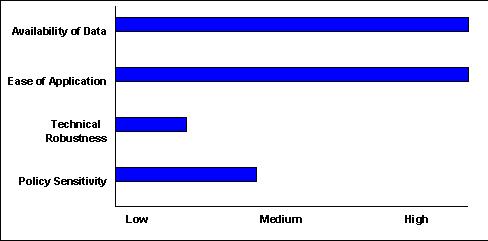
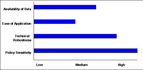
Many areas have implemented inspection and maintenance (I/M) programs to reduce mobile source emissions. Many of the choices for these I/M program specifications are at the discretion of the local agency depending upon the severity of the air pollution problem and the air pollutant of concern. The types of vehicles in the program as well as the types of I/M program may have significant impacts on the estimated emission rates. For example, areas that have employed the most stringent level of I/M program (IM240) have found on-road emission reductions for CO of 45%, hydrocarbon (HC) as large as 35%, and up to 12% for NO_x relative to conditions without the I/M program.^[16]For the more minimal I/M programs (biennial emission idle test), reduction benefits are estimated at 19% for CO, 17% for HC, and 0.5% for NO_x. Thus, the choice of program may have potentially significant changes in emission totals.

MOBILE6 is capable of modeling the impact of up to seven different exhaust and evaporative emission I/M programs on emission factors. By defining multiple I/M emission reduction programs, the user can model different requirements on different types and ages of vehicles or different requirements in different calendar years. MOBILE6 also allows users to enter a number of I/M program parameters to better model specific I/M program features. These parameters include:

• Ability to model annual or biennial I/M programs.
• Ability to model Idle, 2500/Idle, acceleration simulation model (ASM), IM240 (an emission test which measures emissions as the vehicle is driven on a dynamometer through a driving cycle taking up to 240 seconds that simulates actual urban driving), and onboard diagnostic (OBD) exhaust I/M programs.
• Ability to model gas cap, fill-pipe pressure test, and OBD check evaporative I/M programs.
• Ability to control model year coverage.
• Ability to control vehicle class coverage (only gasoline-fueled vehicles can be modeled for I/M).
• Ability to vary the failure rate of the exhaust I/M program for pre-1981 model year vehicles.
• Ability to vary the compliance rate of the I/M program.
• Ability to vary the waiver rate of the I/M program.
• Ability to vary the "cutpoints" (which determine whether a vehicle passes or fails an I/M test) by pollutant, vehicle type, and age used in an IM240 program.
• Ability to account for the effect of exempting old vehicles from program requirements.
• Ability to account for the effect of exempting new vehicles from program requirements
• Ability to eliminate the effects of technician training on exhaust I/M performance.

In addition, the mere presence of an I/M program is expected to act as a deterrent to tampering. Thus, in areas with an I/M program, MOBILE6 will reduce the tampering rates even if there is no anti-tampering program. All 1996 and newer model year vehicles are assumed to have negligible tampering effects in MOBILE6. As a result, there is no tampering reduction benefit associated with the 1996 and newer vehicles.

Addressing I/M Participation

Method 1: Apply Type of I/M Program to Area of Analysis

Description

This methodology uses the local I/M program requirements to define the on-road vehicle fleet that is participating in I/M programs. The approach allows the user to define the local I/M program through the application of the MOBILE6 model. For regions that have significant numbers of vehicles subject to other I/M programs, the MOBILE6 model will need to be applied separately for each I/M program.

Method Applicability

This method is most applicable in a nonattainment or maintenance area where the I/M participation rate in the on-road vehicle fleet is essentially the same as the percentage of vehicles registered in the jurisdiction subject to I/M. In regions where a significant portion of the on-road fleet is from outside the local I/M area, an estimate must be made for the fraction of those vehicles outside the local region (see Method #2).

Data Sources and Procedures

This approach involves running the local specific I/M program requirements through the MOBILE6 model to estimate the effects of the I/M program. If, through the use of local survey data, a significant fraction of the on-road fleet is found to be registered outside the jurisdiction of the local I/M program then the procedure should be modified, as described in Method #2.

In order to forecast emissions, the analysis can account for a change in the counties or local areas where I/M programs will be required in the future. The extent to which I/M program requirements change in the future is an important factor that will affect estimates of future emissions.

Advantages

• Uses the local specific I/M program requirements as defined in local regulations.
• Approach is straightforward and would generally be considered an acceptable approach providing it can be demonstrated that the approach is representative.
• Relatively simple to apply and can be modified easily to account for non-I/M effects through the use of survey data.

Limitations

• The local I/M participation rate may be an invalid representation of the on-road fleet. For example, a number of vehicles from outside the region may pass through the local area, particularly in donut shaped areas, and may therefore cause the local I/M participation rate not to be representative of the local on-road emission rate.
• If survey data is used to estimate the on-road fleet fraction outside the local I/M program control, it may not be representative if an inadequate number of survey days are sampled.

Example Location

This methodology has been applied in both Pennsylvania's Berks County and Wisconsin's Bay Lake Regional Planning Commission.

In Berks County the I/M program began in 2003 for LDGV and LDGT vehicles only. 1996 and newer vehicles had their OBD computer checked, for 1975 to 1995 model year cars an anti-tampering program with seven inspections is performed and for all years a gas cap pressure check is done.

For Wisconsin, emission factors included different model year vapor recovery programs and more basic inspection maintenance procedures. Five vehicle classes were subject to the program: LDGV, LDGT (1 thru 4), and HDGV2B.

References:

Bay-Lake Regional Planning Commission, Wisconsin DOT, and Wisconsin Department of Natural Resources, Assessment of conformity of the Year 2025 Sheboygan Area Transportation and the 2004-2007 Sheboygan Metropolitan Planning Area Transportation Improvement Program (TIP) with Respect to the State of Wisconsin Air Quality Implementation Plan, Fall 2003.

Michael Baker, Jr., Inc., "The 2002 Pennsylvania Statewide Inventory, Using MOBILE6, An Explanation of Methodology," November 2003.

Addressing I/M Participation

Method 2: Use Accident or Other Data Sources to Estimate Proportion of Traffic Subject to I/M

Description

This methodology uses vehicle accident data, or other vehicle data, to estimate the proportion of vehicles in the on-road vehicle fleet that are participating in Inspection & Maintenance (I/M) programs. The approach is unique in that it accounts for the fact that some vehicles traveling in a jurisdiction are registered in another jurisdiction that may not be subject to the same requirements.

Method Applicability

This method is most applicable in a nonattainment or maintenance area where there is reason to believe that the I/M participation rate in the on-road vehicle fleet is significantly different than the percentage of vehicles registered in the jurisdiction subject to I/M (for example, if a jurisdiction does not have an I/M program but a considerable portion of vehicles in the on-road fleet come from other jurisdictions that do, or alternatively, if the jurisdiction has an I/M program and considerable traffic comes from other jurisdictions that do not). This would be particularly important where an I/M program is not statewide and if there is a high level of inter-county or interstate travel.

Data Sources and Procedures

This approach involves using accident data in order to estimate the proportion of vehicles in the on-road fleet that are from jurisdictions subject to I/M program requirements. Accident data are used to determine the county in which vehicles on the road are registered. Based on place of registration, the proportion of vehicles on the road that are subject to I/M programs can be determined.

The MOBILE model is run twice-once with an I/M program and once without an I/M program. A weighted emissions factor is then calculated by multiplying the MOBILE emissions factor with I/M by the percent of vehicles from jurisdictions subject to I/M, plus the MOBILE emissions factor without I/M by the percent of vehicles from jurisdictions without I/M requirements.

To forecast emissions, the analysis can account for a change in the counties where I/M programs will be required in the future. The extent to which I/M program requirements change in the future is an important factor that will affect estimates of future emissions.

Advantages

• Uses a readily available source of data on a county-by-county level. Virtually all counties collect accident data due to its obvious uses related to improving safety in high accident areas.
• Use of the data to estimate the proportion of vehicles subject to I/M is an innovative approach to using existing data for new purposes.
• Relatively simple to operationalize and improves the quality of data used in analysis (i.e., national defaults or local inputs).

Limitations

• Accident data may not provide a valid representation of the proportion of in area vs. out-of-area vehicles.
• The quality of the accident data may create biases. For example, if many accidents occur at nighttime, the mix of vehicles on the road could be very different than during an average day.

Example Location

This methodology has been applied in North Carolina. This methodology was selected since an I/M program currently is limited to nine counties and there is significant county-to-county commuting. The NCDOT assumes that the I/M program in the State will be in force in 48 counties in 2007.

This methodology was used across North Carolina for six urban and six rural road types. It was used primarily for adjusting the vehicle classification mix to reflect the change in fleet mix for higher light-duty truck fraction than the national average using recent historical HPMS data.

References:

Phone conversation with Behshad Norowzi, North Carolina DOT, bnorowzi@dot.state.nc.us), February 17, 2004.

^[15] USEPA, 2002. "Sensitivity Analysis of MOBILE6.0", Assessment and Standards Division, Office of Transportation and Air Quality, EPA420-R-02-035, December 2002.

^[16] Evaluating Vehicle Emissions Inspection and Maintenance Programs, Committee on Vehicle Emission Inspection and Maintenance Programs, Transportation Research Board, National Research Council, National Academy of Press, 2001. ISBN 0-309-07446-0.