U.S. Department of Transportation
Federal Highway Administration
1200 New Jersey Avenue, SE
Washington, DC 20590
202-366-4000
Federal Highway Administration Research and Technology
Coordinating, Developing, and Delivering Highway Transportation Innovations
| REPORT |
| This report is an archived publication and may contain dated technical, contact, and link information |
|
| Publication Number: FHWA-HRT-11-060 Date: November 2011 |
Publication Number: FHWA-HRT-11-060 Date: November 2011 |
The corrosion of steel reinforcement in concrete is a destructive process for both the steel and the concrete. The corrosion products of steel occupy several times the volume of solid steel, resulting in cracking and spalling of the concrete cover once a sufficient amount of corrosion loss has occurred. Several prior studies have worked to establish a relationship between corrosion loss and cracking of concrete cover for uncoated conventional reinforcement.(68-71) In addition, Torres-Acosta and Sagues examined the effects of localized corrosion, although the corroding areas were much larger than the area typically exposed due to damage to ECR.(71)
Limited research has been performed on the amount of corrosion loss required to crack concrete for galvanized reinforcement. Sergi, Short, and Page found that the corrosion product of zinc is often zinc oxide.(73) The volume of zinc oxide is only 1.5 times that of solid zinc, whereas the volume of ferric oxide is 3 times that of solid steel, indicating that the corrosion loss required to crack concrete for specimens with galvanized reinforcement should be greater than the corrosion loss required to crack concrete with conventional reinforcement.(74,75) However, under certain conditions, zinc can also form zinc hydroxychloride II, which has 3.6 times the volume of solid zinc.(73,74) The formation of zinc hydroxychloride II will result in corrosion losses for galvanized reinforcement at the onset of cracking similar to those observed for conventional reinforcement. Rasheeduzzafar et al. studied conventional and galvanized reinforcement cast in concrete with chloride contents at casting ranging from 2.4 to 19.2 kg/m3 (4 to 32 lb/yd3).(76) Rasheeduzzafar et al. found specimens containing galvanized reinforcement took longer to crack concrete than specimens containing conventional reinforcement; however, the corrosion loss at crack initiation was not determined.
The research described in this appendix examines the corrosion losses required to crack concrete cover for conventional, galvanized, and damaged epoxy-coated reinforcement. Specimens with conventional and galvanized reinforcement were tested at varying covers to establish a relationship between corrosion loss and cracking for conventional and galvanized reinforcement. ECR was tested at 25-mm (1-inch) cover with varying damage patterns to determine the effect of the damaged area on corrosion loss required to crack concrete. Two- and three-dimensional finite element models were created to test the corrosion loss to crack concrete for multiple combinations of cover and damaged area. The results from the finite element models are compared with experimental results from this and other studies, and an expression is developed relating damaged area, concrete cover, and corrosion loss to cause cracking.
The mixture proportions used in the concrete for all specimens are shown in table 57. The materials used are as follows:
The mixture includes salt equivalent to 2 percent chlorides by weight of cement to destabilize the passive layer of the reinforcement and increase the ionic conductivity of the concrete. The salt is dissolved in the mix water prior to casting.
Table 57. Mix proportions for cracking specimens.
Cement, kg/m3 |
Water, kg/m3 |
Fine Aggregate, kg/m3 |
Coarse
Aggregate, kg/m3 |
Sodium Chloride,
kg/m3 |
Air Entraining
Agent, |
|---|---|---|---|---|---|
356 (598) |
160 (269) |
854 (1,435) |
883 (1,484) |
11.7 (19.8) |
2.66 (68.9) |
The following materials are used in the cracking tests described in this appendix:
A schematic of the cracking specimens is shown in figure 222. Cracking specimens are beam specimens, 152 mm (6 inches) wide by 305 mm (12 inches) long. Specimen height is dependent on the concrete cover. The top bar is the test bar and consists of conventional, galvanized, or epoxy-coated reinforcement. The bottom bars are pickled 2205 duplex stainless steel. All bars are No. 16 (No. 5) reinforcing steel. Specimens are connected to a power supply to drive corrosion on the test bar and are kept ponded with deionized water.

Figure 222. Illustration. Cracking specimen.
A total of 34 specimens were tested in five series. Series 1 consisted of beams with conventional and galvanized reinforcement with 25-mm (1-inch) concrete cover. Series 2 consisted of beams with conventional and galvanized reinforcement with 13-mm (0.5-inch) concrete cover. Series 3 tested conventional and galvanized reinforcement with 51-mm (2-inch) cover. Series 4 tested damaged ECR with 25-mm (1-inch) concrete cover. Series 5 tested two specimens with galvanized reinforcement and 25-mm (1-inch) cover, with specimens removed from testing at crack initiation. Testing continued on series 1, 2, and 3 until the crack reached a width of 0.508 mm (0.02 inches). Testing continued on series 4 until the crack spanned the full length of the specimen because the lower corrosion rate of specimens containing ECR made it impractical to continue the test until the crack reached a width of 0.508 mm (0.02 inches).
The test begins 14 days after the specimens are cast. During the test, the current to each specimen is measured daily. Dividing the measured current by the surface area of the test bar (or the damaged area for ECR) gives the corrosion current density, which is used to determine corrosion rate using Faraday's equation (see chapter 2). Specimens are monitored daily for staining and cracking. The corrosion loss at staining, crack initiation, and propagation of the crack to the full specimen length are recorded. In addition, the crack width as a function of corrosion loss is tracked for specimens with conventional and galvanized reinforcement.
Specimen fabrication for cracking specimens follows the preparation procedure for bench-scale specimens outlined in chapter 2, with two exceptions. ECR is damaged in either a two-hole or two half-ring pattern, as shown in figure 223 and figure 224. Specimens are also cured in molds for 14 days as opposed to the curing procedure used for bench-scale specimens.

Figure 223. Illustration. Damage patterns for ECR with two holes.

Figure 224. Illustration. Damage patterns for ECR with two half-rings.
The test program is summarized in table 58. The conventional and galvanized reinforcement were tested with 13-mm (0.5-inch), 25-mm (1-inch), and 51-mm (2-inch) concrete covers. The galvanized reinforcement had a nominal coating thickness of 0.15 mm (6 mil). The ECR, with coating thickness ranging from 0.20 to 0.27 mm (8 to 10.5 mil) and an average of 0.25 mm (9.7 mil), was tested using a 25-mm (1-inch) cover with two damage patterns, as previously described.
Table 58. Corrosion loss to cause cracking, number of specimens in test program.
System |
Cover |
||
|---|---|---|---|
13 mm |
25 mm |
51 mm |
|
Uncoated bars (Conv.) |
4 |
4 |
4 |
Galvanized bars (Zn) |
4 |
6a |
4 |
ECR-2 hole damage pattern |
|||
Horizontal alignment (ECR-2h-H) |
- |
2 |
- |
Vertical alignment (ECR-2h-V) |
- |
2 |
- |
ECR-2 ring damage pattern |
|||
Horizontal alignment (ECR-2r-H) |
- |
2 |
- |
Vertical alignment (ECR-2r-V) |
- |
2 |
- |
- No data.
a Two specimens removed from testing at crack initiation.
To further study the relationship between corrosion loss and cracking, two- and three-dimensional finite element models were created using ABAQUS 6.9.(77) The two-dimensional models were used to model uniform corrosion of a reinforcing bar. The three-dimensional models were tested with uniform corrosion over the entire bar, as well as with areas of localized corrosion. The model represents a slab with mirror symmetry about the axis of the reinforcement (see figure 225). The crack is assumed to propagate along the vertical boundary of the model centered on the reinforcing bar. A series of nonlinear springs were used to provide horizontal restraint along the plane of the crack to represent the nonlinear behavior of the concrete as it cracks.

Figure 225. Illustration. Two-dimensional finite element model of concrete to measure cracking behavior.
The properties of the springs were based on measurements of fracture energy of concrete. Darwin et al. tested notched beams in center-point loading.(78) Fracture energy was calculated by determining the area under the load-deflection curves for each specimen. Darwin et al. found that for concretes older than 5 days, fracture energy is governed by coarse aggregate properties and is independent of w/c ratio, compressive strength, and age of concrete. The spring properties were adjusted to provide a fracture energy of 61 N/m (0.35 lb/in), comparable to the value reported by Darwin et al.(78) The initial stiffness of the springs provided an elastic modulus of 27.6 GPa (4,000 ksi) and a peak tensile stress of 2.76 MPa (400 psi). The spring behavior for a spring density of 6,200 springs/m2 (4 springs/in2) is shown in figure 226.
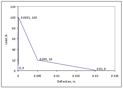
1 lb = 2.228 N
1 inch = 25.4 mm
Figure 226. Graph. Load-deflection behavior for nonlinear spring model, spring density of 6,200 springs/m2 (4 springs/in2).
Material away from the plane of the crack was assumed to be
linear and elastic, with an elastic modulus of 27.6 GPa (4,000 ksi) and a
Poisson's ratio of 0.2. Corrosion was assumed to occur uniformly over the
entire surface of the conventional and galvanized bars and over the localized
damaged regions of the epoxy-coated bars. The buildup of corrosion products was
represented by applying a uniform deflection
normal to the reinforcing bar surface. The volume ratio of corrosion products
to corrosion loss n was assumed to be 3.0 based on work by Suda et al.(75) A visible crack was assumed to have
formed when the horizontal deflection at the top surface of the model (point A
in figure 225) reached 25 ![]() m (1.0 mil). With the model
symmetry, this corresponds to a 50-
m (1.0 mil). With the model
symmetry, this corresponds to a 50-![]() m (2.0-mil)-wide crack. The displacement at the surface of the concrete at
the location of the reinforcing bar required to cause the formation of
the crack (
m (2.0-mil)-wide crack. The displacement at the surface of the concrete at
the location of the reinforcing bar required to cause the formation of
the crack (![]() crit) was
converted to a corrosion loss (xcrit) using the equation in figure
227. The term in the denominator (n-1) accounts for the volume of the
reinforcing bar that is converted to corrosion product.
crit) was
converted to a corrosion loss (xcrit) using the equation in figure
227. The term in the denominator (n-1) accounts for the volume of the
reinforcing bar that is converted to corrosion product.
![]()
Figure 227. Equation. Corrosion loss conversion.
Figure 228 and figure 229 show typical finite element model meshes used for the two- and three-dimensional models. The model dimensions are shown in figure 225. For the two-dimensional finite element models, concrete covers of 6.4, 13, 19, 25, 38, 51, 76, and 102 mm (0.25, 0.5, 0.75, 1, 1.5, 2, 3, and 4 inches) and bar diameters of 13, 19, and 25 mm (0.5, 0.75, and 1 inches) were evaluated. For the three-dimensional finite element models, concrete covers of 51 and 76 mm (2 and 3 inches) and bar diameters of 13, 19, and 25 mm (0.5, 0.75, and 1 inches) were used. The two-dimensional model had a unit length, and the three-dimensional model had a length of 508 mm (20 inches).
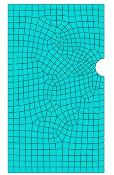
Figure 228. Illustration. Two-dimensional finite element analysis model.
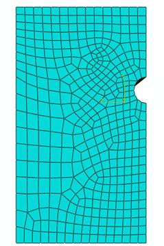
Figure 229. Illustration. Three-dimensional finite element analysis model (end view).
Trial models were run for both the two- and three-dimensional models to determine the effect of mesh type on model performance (see table 59 and table 60). In both cases, the mesh type had no significant effect on the model performance, so the default meshes for the two- and three-dimensional models (quad-dominated and hex, respectively) were used.
Table 59. Effect of two-dimensional element type on corrosion loss.
Mesh Type |
Corrosion Loss
to Produce a 50- |
|---|---|
Quad |
38.99 |
Quad-dominated |
38.48 |
Tri |
38.74 |
1 ![]() m = 0.0394 mil
m = 0.0394 mil
Table 60. Effect of three-dimensional element type on corrosion loss.
| Mesh Type | Corrosion Loss
to Produce a 50- |
|---|---|
Hex |
64.5 |
Hex-dominated |
64.2 |
Wedge |
64.8 |
Tet |
65.4 |
1 ![]() m = 0.0394 mil
m = 0.0394 mil
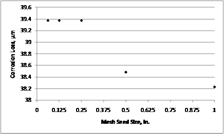
Trial models were also run to determine the effect of mesh seed size on model performance. The mesh seed size was increased until the finite element model results were affected (see figure 230). A 6.4 mm (0.25-inch) mesh was chosen, as it was the largest mesh size for which the finite element model results were not affected.
1 ![]() m = 0.0394 mil
m = 0.0394 mil
Figure 230. Graph. Effect of mesh seed size on corrosion loss required
to produce a 50-![]() m (2-mil) crack.
m (2-mil) crack.
The two-dimensional model was used to analyze uniform corrosion over the entire bar surface. For the three-dimensional model, three damage patterns were analyzed for each combination of cover and bar diameter, as shown in figure 231. The first damage pattern simulates corrosion along the entire circumference of the bar. Models with this damage pattern are designated FR (full ring corrosion pattern). The second damage pattern simulates corrosion along half the bar circumference and is designated HR. The third damage pattern simulates corrosion along one-quarter of the bar circumference and is designated QR. The length of the FR damage pattern along the bar ranged from 3.2 to 508 mm (0.125 to 20 inches). The length of the HR damage pattern along the bar ranged from 3.2 to 203 mm (0.125 to 8 inches), and the length of the QR damage pattern along the bar ranged from 1.6 to 203 mm (0.0625 to 8 inches).

Figure 231. Illustration. Cross section of bar damage patterns for three-dimensional finite element models: full ring, half ring, and quarter ring.
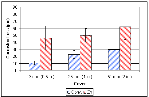
The values of corrosion loss to initiate cracking for
conventional and galvanized reinforcement are shown in figure 232, with the
standard deviation represented by error bars. For all concrete covers,
galvanized reinforcement required significantly greater corrosion losses to
crack the concrete cover than did conventional reinforcement. For 13-mm
(0.5-inch) cover, conventional reinforcement required an average corrosion loss
of 10.6 ![]() m
(0.417 mil) to crack the concrete cover,
compared to 45.9
m
(0.417 mil) to crack the concrete cover,
compared to 45.9 ![]() m (1.81 mil) for galvanized
reinforcement. For 25-mm (1-inch) cover, conventional reinforcement required
an average corrosion loss of 22.4
m (1.81 mil) for galvanized
reinforcement. For 25-mm (1-inch) cover, conventional reinforcement required
an average corrosion loss of 22.4 ![]() m (0.882 mil) to crack the concrete cover, compared to 49.7
m (0.882 mil) to crack the concrete cover, compared to 49.7 ![]() m (1.91 mil)
for galvanized reinforcement, and for 51‑mm (2-inch) cover, conventional reinforcement required
an average corrosion loss of 29.7
m (1.91 mil)
for galvanized reinforcement, and for 51‑mm (2-inch) cover, conventional reinforcement required
an average corrosion loss of 29.7 ![]() m (1.17 mil) to
crack the concrete cover, compared to 68.0
m (1.17 mil) to
crack the concrete cover, compared to 68.0 ![]() m (2.68 mil) for galvanized
reinforcement. For conventional
reinforcement, increasing the cover from 13 to 51 mm (0.5 to 2 inches) nearly tripled
the corrosion loss required to crack concrete from 10.6 to 29.7
m (2.68 mil) for galvanized
reinforcement. For conventional
reinforcement, increasing the cover from 13 to 51 mm (0.5 to 2 inches) nearly tripled
the corrosion loss required to crack concrete from 10.6 to 29.7 ![]() m (0.417 to 1.17 mil), an increase of 19.1
m (0.417 to 1.17 mil), an increase of 19.1 ![]() m (0.752 mil). For
galvanized reinforcement, the loss increased by 48 percent from 45.9 to
68.0
m (0.752 mil). For
galvanized reinforcement, the loss increased by 48 percent from 45.9 to
68.0 ![]() m
(1.81 to 2.68 mil), an increase of 22.1
m
(1.81 to 2.68 mil), an increase of 22.1 ![]() m (0.870 mil).
m (0.870 mil).
1 ![]() m = 0.0394 mil
m = 0.0394 mil
Figure 232. Graph. Average corrosion loss required to crack concrete for specimens with conventional and galvanized reinforcement.
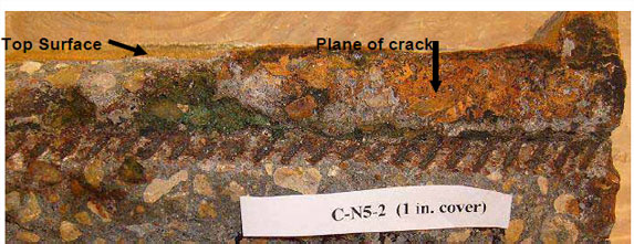
Autopsy results from all specimens with conventional reinforcement showed heavy corrosion losses over the entire bar surface (see figure 233 and figure 234). Staining was apparent in the concrete surrounding the reinforcement. Figure 235 shows a side view of the concrete around the reinforcement split along the plane of the crack. Orange corrosion products are visible in regions where the staining reached the surface. In figure 236, greenish-black corrosion products are visible in regions isolated from the atmosphere. All photos were taken immediately after autopsy.
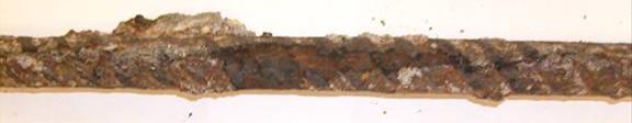
Figure 233. Photo. Top side of bar in specimen Conv.-3, 51-mm (2-inch) cover, after autopsy.
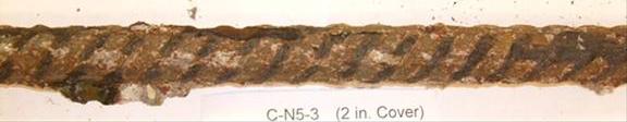
Figure 234. Photo. Bottom side of bar in specimen Conv.-3, 51-mm (2-inch) cover, after autopsy.
![]()
Figure 235. Photo. Side view of specimen Conv.-2, 25-mm (1-inch) cover, after autopsy (plane of crack visible above reinforcement).
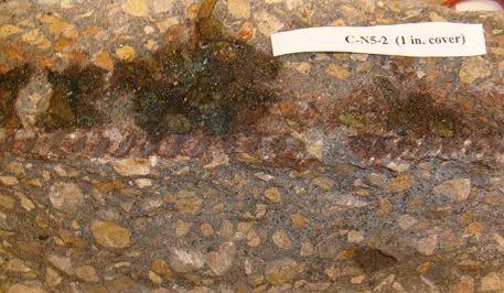
Figure 236. Photo. Top view of specimen Conv.-2, 25-mm (1-inch) cover, after autopsy.
The autopsy found that galvanized reinforcement exhibited signs of pitting corrosion. Some regions of the test bar exhibited heavy corrosion products, while in other sections, the galvanized coating was unaffected (see figure 237 and figure 238). Most of the uncorroded regions were located on the top face of the bar, a result of the bottom side of the bar having more even exposure to the ions migrating from the bottom bars. Measurements with a coating thickness gauge showed no significant loss in the areas that appear uncorroded. Visual estimations of uncorroded surface areas were performed on all bars after autopsy, and results appear in table 61. The bars with 13-mm (0.5‑inch) cover showed the greatest average uncorroded area, 29 percent, likely due to the decreased cover interfering with ion transport to the top side of the bar. The bars with 25- and 51-mm (1- and 2-inch) cover showed average uncorroded areas of 6 and 13 percent, respectively. The corrosion products on the concrete surrounding the galvanized reinforcement resembled those seen in specimens with conventional reinforcement, indicating that the bulk of corrosion products applying pressure to the surrounding concrete are corrosion products of iron and not those of zinc (see figure 239 and figure 240).
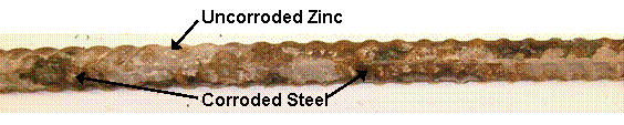
Figure 237. Photo. Top side of bar in specimen Zn-2, 25-mm (1-inch) cover, after autopsy.
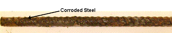
Figure 238. Photo. Bottom side of bar in specimen Zn-2, 25-mm (1-inch) cover, after autopsy.
Table 61. Estimated uncorroded surface area of galvanized reinforcement.
| Specimen | Estimated Uncorroded Area, percent | ||
|---|---|---|---|
| Cover | |||
| 13 mm (0.5 inch) | 25 mm (1 inch) | 51 mm (2 inch) | |
Zn-1 |
30 |
8 |
5 |
Zn-2 |
30 |
5 |
10 |
Zn-3 |
40 |
5 |
50 |
Zn-4 |
15 |
5 |
30 |
Average |
29 |
6 |
13 |
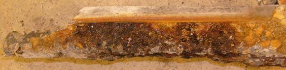
Figure 239. Photo. Side view of specimen Zn-4, 25-mm (1-inch) cover, after autopsy.
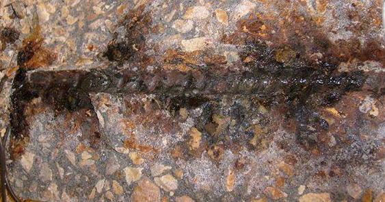
Figure 240. Photo. Top view of specimen Zn-4, 25-mm (1-inch) cover, after autopsy.
To determine if the pitting observed on galvanized reinforcement was also present at crack initiation, two additional specimens with galvanized reinforcement and 25-mm (1-inch) cover were cast and autopsied at the onset of cracking. Greenish-black corrosion products were visible along the crack at the upper surface of the specimens (see figure 241). The corrosion products turned orange about 2 h after exposure to air. The autopsy revealed pitting and localized corrosion on the bars similar to that observed in the specimens autopsied after the crack had propagated and widened (see figure 242 and figure 243). As previously discussed, uncorroded regions were more common on the top than the bottom side of the test bar (see figure 244). These results suggest that cracking of the concrete due to corrosion of the galvanized reinforcement did not result due to the buildup of zinc corrosion products but rather due to the formation of corrosion products from the intermetallic steel-zinc layers or from the underlying steel.
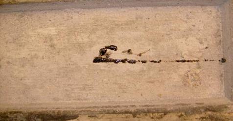
Figure 241. Photo. Staining on surface at crack initiation in galvanized reinforcement specimen, 25-mm (1‑inch) cover.
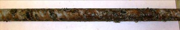
Figure 242. Photo. Top side of galvanized reinforcement, 25-mm (1-inch) cover, after autopsy at crack initiation.
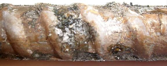
Figure 243. Photo. Detail of top side of galvanized reinforcement, 25-mm (1-inch) cover, after autopsy at crack initiation.
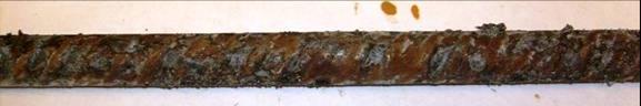
Figure 244. Photo. Bottom side of galvanized reinforcement, 25-mm (1-inch) cover, after autopsy at crack initiation.
The corrosion losses required to crack concrete cover for specimens containing damaged ECR are shown in table 62. The losses are presented based on both the total area of the bar and the damaged (exposed) area in the epoxy. The bars with two half-rings had a nominal exposed area ten times greater than the bars with two holes in the epoxy; however, autopsy results revealed significant blistering on bars with holes in the epoxy (see figure 245). Blistering was also present on the bars with the half-rings but was less severe and exposed less than the area exposed by the rings. Table 62 reflects an estimate of the increased exposed area from the blistered regions for all specimens. Ignoring the blistered regions, specimens with two half-rings had an exposed area of 150.8 mm2 (0.234 in2) and specimens with two holes had an exposed area of 15.8 mm2 (0.024 in2).
Table 62. Average corrosion loss to crack concrete cover for specimens with ECR.
| Specimen | Exposed Area (Including Blisters), mm2 | Corrosion Loss Based on Total Area, |
Corrosion Loss Based on Exposed Area, |
|---|---|---|---|
ECR-2 hole damage pattern |
|||
ECR-2h-H-1 |
188.3 |
10.14 |
730 |
ECR-2h-H-2 |
233.5 |
10.10 |
587 |
ECR-2h-H Average |
10.12 |
659 |
|
ECR-2h-V-1 |
181.8 |
11.67 |
874 |
ECR-2h-V-2 |
201.1 |
7.58 |
510 |
ECR-2h-V Average |
9.70 |
692 |
|
ECR-2 ring damage pattern |
|||
ECR-2r-H-1 |
208.9 |
6.07 |
421 |
ECR-2r-H-2 |
234 |
5.87 |
363 |
ECR-2r-H Average |
5.97 |
392 |
|
ECR-2r-V-1 |
254 |
6.22 |
354 |
ECR-2r-V-2 |
208.9 |
6.15 |
426 |
ECR-2r-V Average |
6.18 |
390 |
|
1 mm2 = 0.00155 in2
1 ![]() m
= 0.0394 mil
m
= 0.0394 mil
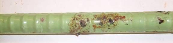
Figure 245. Photo. Test bar from specimen ECR-2h-V-2.
Table 62 shows no significant difference in the corrosion loss required to crack the concrete cover between the specimens with the damage pattern oriented horizontally or vertically. The corrosion losses on both the total and exposed areas indicate that the corrosion loss required to crack the concrete cover increases as exposed area decreases. Based on total and exposed area including blisters, the specimens with two holes in the epoxy required somewhat less than twice the corrosion loss to crack the concrete cover as the specimens with two half-rings in the epoxy.
Figure 246 shows a specimen at crack initiation. Figure 247 shows a specimen with the crack spanning the length of the specimen. No specimens containing ECR showed signs of surface staining during the test. After testing, however, staining was observed on the concrete surrounding the damaged regions in the epoxy when the specimens were autopsied (see figure 248 and figure 249).
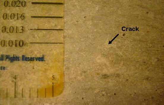
Figure 246. Photo. Crack initiation in specimen ECR-2r-H-2.
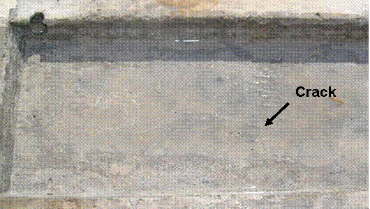
Figure 247. Photo. Crack propagation in specimen ECR-2h-V-1.
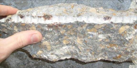
Figure 248. Photo. Concrete surrounding test bar from specimen ECR-2h-V-1.
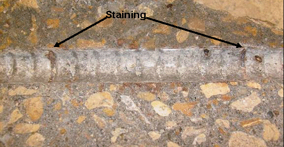
Figure 249. Photo. Concrete surrounding test bar from specimen ECR-2r-H-2.
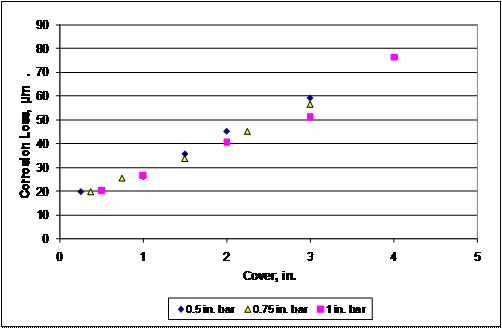
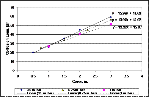
The corrosion losses that
cause a 50-![]() m (2-mil)-wide crack to form
at the surface of the specimen based on the two-dimensional finite
element analyses are shown in table 63. The corrosion losses are plotted as a
function of concrete cover in figure 250. The results suggest a linear
relationship (for covers between 6 and 102 mm (0.25 and 4 inches)) between
concrete cover and corrosion loss required to cause cracking. A slight
dependence on bar diameter is also noted; figure 251 shows best-fit lines for
each of the three bar diameters over the range of covers from 19 to 76 mm
(0.75 to 3 inches).
m (2-mil)-wide crack to form
at the surface of the specimen based on the two-dimensional finite
element analyses are shown in table 63. The corrosion losses are plotted as a
function of concrete cover in figure 250. The results suggest a linear
relationship (for covers between 6 and 102 mm (0.25 and 4 inches)) between
concrete cover and corrosion loss required to cause cracking. A slight
dependence on bar diameter is also noted; figure 251 shows best-fit lines for
each of the three bar diameters over the range of covers from 19 to 76 mm
(0.75 to 3 inches).
Table 63. Finite element results for two-dimensional model.
| Cover, mm | Bar Diameter, mm | Corrosion Loss to
Crack Concretea, |
|---|---|---|
6.4 |
12.7 |
19.7 |
13 |
12.7 |
20.3 |
25 |
12.7 |
26.0 |
38 |
12.7 |
35.6 |
51 |
12.7 |
45.1 |
76 |
12.7 |
59.5 |
9.5 |
19 |
19.7 |
19 |
19 |
25.4 |
38 |
19 |
33.7 |
57 |
19 |
45.1 |
76 |
19 |
56.5 |
13 |
25.4 |
20.3 |
25 |
25.4 |
26.7 |
51 |
25.4 |
40.6 |
76 |
25.4 |
51.1 |
102 |
25.4 |
76.2 |
1 mm = 0.039 inches
1 ![]() m
= 0.0394 mil
m
= 0.0394 mil
a 50-![]() m (0.002-inch) crack width.
m (0.002-inch) crack width.
1 ![]() m = 0.0394 mil
m = 0.0394 mil
1 inch = 25.4 mm
Figure 250. Graph. Corrosion loss to crack concrete versus cover for two-dimensional finite element model.
1 ![]() m = 0.0394 mil
m = 0.0394 mil
1 inch = 25.4 mm
Figure 251. Graph. Corrosion loss to crack concrete versus cover showing effect of bar diameter for two-dimensional finite element model.
Table 63 and figure 251 show that as cover increases, bars with smaller diameters require somewhat greater corrosion losses to crack concrete than bars with larger diameters for covers between 25 and 76 mm (1 and 3 inches). An analysis of the data suggests the equation in figure 252 as a best-fit expression. The English equivalent is presented in figure 253.
![]()
Figure 252. Equation. Suggested best-fit in SI units.
![]()
Figure 253. Equation. Suggested best-fit in English units.
Where:
xcrit =
Corrosion loss at crack initiation, ![]() m or mil.
m or mil.
C = Cover, mm or inches.
D = Bar diameter, mm or inches.
To verify the accuracy of the two-dimensional finite element model, the results obtained from the model are compared with experimental results presented in this appendix along with experimental results obtained by Saeki et al., Rasheeduzzafar et al., Alonso et al., and Torres-Acosta and Sagues for corrosion along the full length of conventional reinforcement. (See references 68, 69, 71, and 79.) The data from these sources are shown in table 64. The experimental data are plotted along with the finite element results in figure 254. Data presented in this appendix are labeled "KU." Other data are identified by the first author. A best-fit line for the results from the finite element model is also shown. While there is much scatter in the experimental data, the corrosion loss required to crack concrete, as predicted by the finite element model, provides an excellent representation of the bulk of the experimental data.
Table 64. Corrosion loss to crack concrete (corrosion along entire bar length).
| Study | Cover, mm | Diameter, mm | Corrosion Loss, |
|---|---|---|---|
Torres-Acosta and Sagues(71) |
39 |
13 |
35.9 |
39 |
13 |
31.1 |
|
Alonso et al.(69) |
20 |
16 |
15 |
15 |
8 |
20 |
|
30 |
16 |
25 |
|
30 |
16 |
28 |
|
30 |
16 |
30 |
|
50 |
16 |
31 |
|
50 |
12 |
51 |
|
70 |
16 |
55 |
|
70 |
10 |
68 |
|
20 |
16 |
25 |
|
20 |
16 |
18 |
|
Rasheeduzzafar et al.(68) |
19 |
13 |
33 |
19 |
13 |
26 |
|
19 |
13 |
34 |
|
38 |
13 |
32 |
|
38 |
13 |
30 |
|
38 |
13 |
47 |
|
38 |
13 |
38 |
|
38 |
13 |
27 |
|
38 |
13 |
27 |
|
50 |
13 |
70 |
|
50 |
13 |
71 |
|
50 |
13 |
74 |
|
50 |
13 |
61 |
|
60 |
13 |
67 |
|
Saeki et al.(79) |
31.75 |
9.5 |
42 |
31.75 |
12.7 |
34 |
|
31.75 |
19 |
23 |
|
31.75 |
25 |
13 |
1 mm = 0.039 inches
1 ![]() m
= 0.0394 mil
m
= 0.0394 mil

1 ![]() m = 0.0394 mil
m = 0.0394 mil
1 inch = 25.4 mm
Figure 254. Graph. Corrosion loss to crack concrete versus cover in two-dimensional finite element model with experimental data.
To determine its accuracy, the results predicted by the equation in figure 252 are compared with experimental results and finite element model results in figure 255.
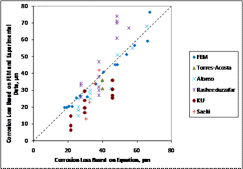
Figure 255. Graph. Corrosion loss to crack concrete for uniform general corrosion based on experimental and finite element results versus predicted corrosion losses using figure 252.
The proposed equation overestimates the corrosion loss
required to crack concrete for most cases in which the actual corrosion loss
required to crack the concrete is less than 45 ![]() m (1.78 mil). An alternate
equation is proposed in figure 256 and figure 257 that provides a somewhat more
conservative estimate of the corrosion loss required to crack concrete (see figure
258).
m (1.78 mil). An alternate
equation is proposed in figure 256 and figure 257 that provides a somewhat more
conservative estimate of the corrosion loss required to crack concrete (see figure
258).
![]()
Figure 256. Equation. Alternate best-fit in SI units.
![]()
Figure 257. Equation. Alternate best-fit in English units.
Where:
xcrit =
Corrosion loss at crack initiation, ![]() m or mil.
m or mil.
C = Cover, mm or inches.
D = Bar diameter, mm or inches.
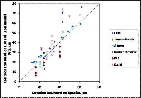
Figure 258. Graph. Corrosion loss to crack concrete for uniform general corrosion based on experimental and finite element results versus predicting corrosion losses using figure 256.
The corrosion losses to cause cracking based on the
three-dimensional finite element model are shown in table 65 and table 66. The
models with a 51-mm (2-inch) cover and a 203-mm (8-inch) and 508-mm (20-inch)
length of bar corroding show similar corrosion losses at crack initiation. The
behavior of the three-dimensional finite element model under full-bar-length (508 mm
(20 inches)) corrosion is compared to that
of the two-dimensional finite element model in figure 259. The corrosion
losses to cause cracking obtained from these models are similar. The differences
in corrosion loss to crack concrete
between two- and three-dimensional models is less than 1 ![]() m (0.039 mil), with the exception of models with a 25-mm
(1-inch)-diameter bar and 76-mm (3‑inch) cover, which show a 2.9-
m (0.039 mil), with the exception of models with a 25-mm
(1-inch)-diameter bar and 76-mm (3‑inch) cover, which show a 2.9-![]() m (0.11-mil) or 5.7 percent difference
in corrosion loss to cause cracking.
m (0.11-mil) or 5.7 percent difference
in corrosion loss to cause cracking.
Table 65. Finite element results for three-dimensional model, 51-mm (2-inch) cover.
| Corrosion Pattern | 13-mm (0.5-in.) Bar Diameter | 19-mm (0.75-in.) Bar Diameter | 25-mm (1-in.) Bar Diameter | |||
|---|---|---|---|---|---|---|
| Exposed Area, mm2 (in2) |
Corrosion Loss at Cracking, |
Exposed Area, mm2 (in2) |
Corrosion Loss at Cracking, |
Exposed Area, mm2 (in2) |
Corrosion Loss at Cracking, |
|
Full Ring |
||||||
508 mm (20 in.) length |
10,134 (15.7) |
46 |
15,201 (23.6) |
43 |
20,268 (31.4) |
40 |
203 mm (8 in.) length |
4,054 (6.28) |
57 |
6,080 (9.42) |
44 |
8,107 (12.6) |
41 |
102 mm (4 in.) length |
2,027 (3.14) |
79 |
3,040 (4.71) |
57 |
4,054 (6.28) |
56 |
51 mm (2 in.) length |
1,013 (1.57) |
159 |
1,520 (2.36) |
133 |
2,027 (3.14) |
80 |
25 mm (1 in.) length |
507 (0.785) |
330 |
760 (1.18) |
254 |
1,013 (1.57) |
144 |
13 mm (0.5 in.) length |
253 (0.392) |
483 |
380 (0.589) |
381 |
507 (0.785) |
281 |
6.4 mm (0.25 in.) length |
127 (0.196) |
659 |
190 (0.295) |
508 |
253 (0.392) |
361 |
3.2 mm (0.125 in.) length |
63.3 (0.098) |
851 |
95 (0.147) |
658 |
127 (0.196) |
502 |
Half Ring |
||||||
102 mm (4 in.) length |
1,013 (1.57) |
178 |
1,520 (2.36) |
152 |
2,027 (3.14) |
88 |
51 mm (2 in.) length |
507 (0.785) |
273 |
760 (1.18) |
229 |
1,013 (1.57) |
150 |
25 mm (1 in.) length |
253 (0.392) |
425 |
380 (0.589) |
347 |
507 (0.785) |
279 |
13 mm (0.5 in.) length |
127 (0.196) |
635 |
190 (0.295) |
502 |
253 (0.392) |
418 |
6.4 mm (0.25 in.) length |
63.3 (0.098) |
904 |
95.0 (0.147) |
704 |
127 (0.196) |
572 |
3.2 mm (0.125 in.) length |
31.7 (0.049) |
1,228 |
47.5 (0.074) |
973 |
63.3 (0.098) |
784 |
Quarter Ring |
||||||
102 mm (4 in.) length |
507 (0.785) |
216 |
760 (1.18) |
191 |
1,013 (1.57) |
170 |
51 mm (2 in.) length |
253 (0.392) |
337 |
380 (0.589) |
292 |
507 (0.785) |
259 |
25 mm (1 in.) length |
127 (0.196) |
546 |
190 (0.295) |
470 |
253 (0.392) |
404 |
13 mm (0.5 in.) length |
63.3 (0.098) |
861 |
95.0 (0.147) |
737 |
127 (0.196) |
622 |
6.4 mm (0.25 in.) length |
31.7 (0.049) |
1,293 |
47.5 (0.074) |
1,090 |
63.3 (0.098) |
890 |
3.2 mm (0.125 in.) length |
15.8 (0.025) |
1,969 |
23.8 (0.037) |
1,562 |
31.7 (0.049) |
1,226 |
1.6 mm (0.0625 in.) length |
7.9 (0.012) |
2654 |
11.8 (0.018) |
2,223 |
15.8 (0.025) |
1,930 |
1 ![]() m = 0.0394 mil
m = 0.0394 mil
Table 66. Finite element results for three-dimensional model, 76-`mm (3-inch) cover.
| Corrosion Pattern | 13-mm (0.5-in.) Bar Diameter | 19-mm (0.75-in.) Bar Diameter | 25-mm (1-in.) Bar Diameter | |||
|---|---|---|---|---|---|---|
| Exposed Area, mm2 (in2) |
Corrosion Loss at Cracking, |
Exposed Area, mm2 (in2) |
Corrosion Loss at Cracking, |
Exposed Area, mm2 (in2) |
Corrosion Loss at Cracking, |
|
Full Ring |
||||||
508 mm (20 in.) length |
10,134 (15.7) |
57 |
15,201 (23.6) |
56 |
20,268 (31.4) |
54 |
203 mm (8 in.) length |
4,054 (6.28) |
102 |
6,080 (9.42) |
152 |
8,107 (12.6) |
83 |
102 mm (4 in.) length |
2,027 (3.14) |
216 |
3,040 (4.71) |
267 |
4,054 (6.28) |
108 |
51 mm (2 in.) length |
1,013 (1.57) |
445 |
1,520 (2.36) |
406 |
2,027 (3.14) |
267 |
25 mm (1 in.) length |
507 (0.785) |
660 |
760 (1.18) |
584 |
1,013 (1.57) |
446 |
13 mm (0.5 in.) length |
253 (0.392) |
927 |
380 (0.589) |
813 |
507 (0.785) |
611 |
6.4 mm (0.25 in.) length |
127 (0.196) |
1,295 |
190 (0.295) |
1,067 |
253 (0.392) |
853 |
3.2 mm (0.125 in.) length |
63.3 (0.098) |
1,689 |
95 (0.147) |
1,321 |
127 (0.196) |
1,116 |
Half Ring |
||||||
102 mm (4 in.) length |
1,013 (1.57) |
368 |
1,520 (2.36) |
356 |
2,027 (3.14) |
328 |
51 mm (2 in.) length |
507 (0.785) |
559 |
760 (1.18) |
521 |
1,013 (1.57) |
483 |
25 mm (1 in.) length |
253 (0.392) |
838 |
380 (0.589) |
762 |
507 (0.785) |
693 |
13 mm (0.5 in.) length |
127 (0.196) |
1,219 |
190 (0.295) |
1,118 |
253 (0.392) |
968 |
6.4 mm (0.25 in.) length |
63.3 (0.098) |
1,676 |
95.0 (0.147) |
1,461 |
127 (0.196) |
1,283 |
3.2 mm (0.125 in.) length |
31.7 (0.049) |
2,261 |
47.5 (0.074) |
1,842 |
63.3 (0.098) |
1,689 |
Quarter Ring |
||||||
102 mm (4 in.) length |
507 (0.785) |
508 |
760 (1.18) |
445 |
1,013 (1.57) |
394 |
51 mm (2 in.) length |
253 (0.392) |
737 |
380 (0.589) |
622 |
507 (0.785) |
610 |
25 mm (1 in.) length |
127 (0.196) |
1,067 |
190 (0.295) |
927 |
253 (0.392) |
902 |
13 mm (0.5 in.) length |
63.3 (0.098) |
1,626 |
95.0 (0.147) |
1,308 |
127 (0.196) |
1,270 |
6.4 mm (0.25 in.) length |
31.7 (0.049) |
2,350 |
47.5 (0.074) |
1,791 |
63.3 (0.098) |
1,702 |
3.2 mm (0.125 in.) length |
15.8 (0.025) |
3,226 |
23.8 (0.037) |
2,502 |
31.7 (0.049) |
2,273 |
1.6 mm (0.0625 in.) length |
7.9 (0.012) |
4,343 |
11.8 (0.018) |
3,543 |
15.8 (0.025) |
3,226 |
1 ![]() m = 0.0394 mil
m = 0.0394 mil
1 ![]() m = 0.0394 mil
m = 0.0394 mil
1 inch = 25.4 mm
Figure 259. Graph. Corrosion loss to crack concrete for uniform general corrosion versus cover for two-and three-dimensional finite element model.
The number of variables studied in the three-dimensional finite element model makes plotting all data points on a single plot impractical. Instead, data subsets holding as many variables constant as possible are analyzed to determine the effect of a variable on the corrosion loss required to crack concrete. Furthermore, corroding area, bar diameter, length of corroding region, and damage pattern are not independent variables-specifying any three variables restricts the fourth to a single value. For this analysis, the effect of cover, bar diameter, corroding area, and corroding length are analyzed with the goal of creating an equation that reduces to figure 256 in the case of general corrosion. Corroding area is expressed as a fraction of the total area of the bar, Af(Af = Acorroding/Abar). Corroding length is expressed as a fraction of the total length of the bar, Lf(Lf = Lcorroding/Lbar).
The corrosion loss to crack concrete is plotted versus exposed area for a 13-mm (0.5-inch)-diameter bar with 51-mm (2-inch) cover in figure 260. A curve of the form xcrit = m(Af)b is fit to the data. Table 67 summarizes the values of m and b for all three-dimensional finite element models. Based on table 67, it may be reasonably assumed the constant b is equal to -0.6, while the constant A is dependent on other variables.
Figure 260. Graph. Corrosion loss to crack concrete versus fraction of exposed area with best-fit line for 13-mm (0.5-inch)-diameter bar and 51-mm (2-inch) cover.
Table 67. Constants m and b for best-fit curve xcrit = m(Af)b to corrosion loss versus Af plots.
| Bar Diameter, mm (inches) | Cover, mm (inches) | m | b |
|---|---|---|---|
13 (0.5) |
51 (2) |
41.11 |
-0.602 |
19 (0.75) |
51 (2) |
34.20 |
-0.597 |
25 (1) |
51 (2) |
26.60 |
-0.600 |
13 (0.5) |
76 (3) |
85.11 |
-0.587 |
19 (0.75) |
76 (3) |
78.97 |
-0.592 |
25 (1) |
76 (3) |
60.65 |
-0.589 |
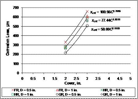
Figure 261 shows the relationship between corrosion loss and cover for all bars with a corroding area of 1,013 mm2 (1.57 in2). Similar plots were analyzed for other exposed areas. For bars with a fixed damage pattern and diameter, increasing the cover from 51 to 76 mm (2 to 3 inches) approximately doubles the corrosion loss required to crack concrete. This suggests that for localized corrosion, the corrosion loss required to crack concrete is proportional to cover squared. For larger corroding areas, the relationship between corrosion loss and cover becomes linear, as shown in figure 252 and figure 256.
1 ![]() m = 0.0394 mil
m = 0.0394 mil
1 inch = 25.4 mm
Figure 261. Graph. Corrosion loss to crack concrete xcrit versus cover C for 1,013-mm2 (1.57-in2) corroding area.
Figure 262 shows the relationship between corrosion loss and fractional corroding length Lf (Lf = Lcorroding/Lbar) for all bars with a corroding area of 1013 mm2 (1.57 in2). Similar plots are analyzed for other lengths. A best-fit power line to the data suggests a relationship between corrosion loss and fractional corroding length to the -0.1 power.
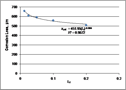
Figure 262. Graph. Corrosion loss to crack concrete xcrit versus Lf with best fit line for 1,013-mm2 (1.57-in2) corroding area.
Based on the data presented, the equations in figure 263 and figure 264 represent a potential relationship between corrosion loss and the variables in this study. The term 3Af -1 is required for localized corrosion and reduces to 1 for general corrosion.

Figure 263. Equation. Potential relationship between corrosion loss and variables in English units.

Figure 264. Equation. Potential relationship between corrosion loss and variables in SI units.
Where:
xcrit =
Corrosion loss at crack initiation, mil or ![]() m.
m.
C = Cover, inches or mm.
D = Bar diameter, inches or mm.
Lf = Fractional length of bar corroding, Lcorroding/Lbar.
Af = Fractional area of bar corroding, Acorroding/Abar.
Figure 265 compares the corrosion losses for the finite element models with the corrosion losses predicted by the equation. There is some scatter, but the equations in figure 263 and figure 264 provide a reasonable match with the results obtained from the finite element model.
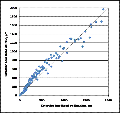
Figure 265. Graph. Corrosion loss to crack concrete for localized corrosion based on the finite element model results versus corrosion losses calculated by the equations in figure 263 and figure 264.
To further verify the accuracy of the equations in figure 263 and figure 264, the corrosion loss predicted by the equation is compared to the experimental data for localized corrosion of ECR, as well as experimental results presented by Rasheeduzzafar et al., Alonso et al., and Torres-Acosta and Sagues, which are summarized in table 68.(68,69,71) Data for generalized corrosion of steel are also included in the analysis to check the accuracy of the equation for bars with large corroding areas. The comparison is presented in figure 266 and figure 267 along with the comparison for the three-dimensional finite element model results shown in figure 265.
Table 68. Results from other research: corrosion loss to crack concrete (localized corrosion).
Cover, mm |
Diameter, mm |
Exposed Area, mm2 |
Bar Area, mm2 |
Exposed Length, mm |
Bar Length, mm |
Corrosion Loss, |
|
|---|---|---|---|---|---|---|---|
Torres-Acosta and Sagues (72) |
27.6 |
21 |
2,105 |
16,757 |
32 |
254 |
48.3 |
27.6 |
21 |
2,105 |
16,757 |
32 |
254 |
66.4 |
|
40.3 |
21 |
2,738 |
20,122 |
42 |
305 |
88.2 |
|
40.3 |
21 |
2,738 |
20,122 |
42 |
305 |
69.6 |
|
65.7 |
21 |
4,486 |
26,785 |
68 |
406 |
76.5 |
|
65.7 |
21 |
4,486 |
26,785 |
68 |
406 |
121.8 |
|
40.3 |
21 |
2,764 |
20,122 |
42 |
305 |
55.2 |
|
40.3 |
21 |
2,764 |
20,122 |
42 |
305 |
68.9 |
|
40.3 |
21 |
1,260 |
13,393 |
19 |
203 |
141.2 |
|
40.3 |
21 |
1,260 |
13,393 |
19 |
203 |
70.6 |
|
40.3 |
21 |
2,738 |
20,122 |
42 |
305 |
60.3 |
|
40.3 |
21 |
2,738 |
20,122 |
42 |
305 |
65.0 |
|
40.3 |
21 |
22,827 |
26,785 |
346 |
406 |
28.4 |
|
40.3 |
21 |
22,827 |
26,785 |
346 |
406 |
7.2 |
|
27.5 |
21 |
1,649 |
26,785 |
25 |
406 |
30.8 |
|
40.3 |
21 |
1,649 |
26,785 |
25 |
406 |
61.6 |
|
45 |
13 |
4,084 |
16,581 |
100 |
406 |
84.0 |
|
45 |
13 |
1,021 |
16,581 |
25 |
406 |
336.0 |
|
38 |
13 |
4,084 |
16,581 |
100 |
406 |
49.8 |
|
38 |
13 |
4,084 |
16,581 |
100 |
406 |
49.8 |
|
13 |
13 |
4,084 |
16,581 |
100 |
406 |
31.1 |
|
13 |
13 |
1,021 |
16,581 |
25 |
406 |
37.3 |
|
13 |
13 |
1,021 |
16,581 |
25 |
406 |
49.8 |
|
13 |
13 |
4,084 |
16,581 |
100 |
406 |
3B2 |
|
28.8 |
13 |
796 |
16,581 |
20 |
406 |
207.4 |
|
30.3 |
13 |
796 |
16,581 |
20 |
406 |
111.7 |
|
39 |
13 |
15,928 |
16,581 |
390 |
406 |
35.9 |
|
39 |
13 |
15,928 |
16,581 |
390 |
406 |
31.1 |
|
39 |
13 |
1,593 |
16,581 |
39 |
406 |
151.6 |
|
39 |
13 |
1,593 |
16,581 |
39 |
406 |
159.6 |
|
39 |
13 |
327 |
16,581 |
8 |
406 |
233.3 |
|
39 |
13 |
327 |
16,581 |
8 |
406 |
272.2 |
|
27.5 |
6.4 |
603 |
8,163 |
30 |
406 |
63.2 |
|
26.5 |
6.4 |
603 |
8,163 |
30 |
406 |
8B3 |
|
39 |
13 |
1,593 |
16,581 |
39 |
406 |
271.2 |
|
39 |
13 |
1,593 |
16,581 |
39 |
406 |
191.5 |
|
39 |
13 |
1,593 |
16,581 |
39 |
406 |
159.6 |
|
39 |
13 |
1,593 |
16,581 |
39 |
406 |
151.6 |
Table 68. Results from other research: corrosion loss to crack concrete (localized corrosion)-Continued.
Cover, mm |
Diameter, mm |
Exposed Area, mm2 |
Bar Area, mm2 |
Exposed Length, mm |
Bar Length, mm |
Corrosion Loss, |
|
|---|---|---|---|---|---|---|---|
Alonso et al.(70) |
19 |
1B6 |
17,448 |
17,448 |
381 |
381 |
15 |
15.2 |
8.0 |
9,550 |
9,550 |
381 |
381 |
20 |
|
30.4 |
16.0 |
19,101 |
19,101 |
381 |
381 |
25 |
|
30.4 |
16.0 |
19,101 |
19,101 |
381 |
381 |
28 |
|
30.4 |
16.0 |
19,101 |
19,101 |
381 |
381 |
30 |
|
49.4 |
15.9 |
19,024 |
19,024 |
381 |
381 |
31 |
|
49.4 |
11.8 |
14,041 |
14,041 |
381 |
381 |
51 |
|
68.4 |
15.5 |
18,558 |
18,558 |
381 |
381 |
55 |
|
68.4 |
9.8 |
11,665 |
11,665 |
381 |
381 |
68 |
|
19 |
1B6 |
17,448 |
17,448 |
381 |
381 |
25 |
|
19 |
1B6 |
17,448 |
17,448 |
381 |
381 |
18 |
|
29 |
38.1 |
91,207 |
91,207 |
381 |
381 |
3 |
|
Rasheeduzzafar et al.(69) |
20 |
13 |
22,462 |
22,462 |
550 |
550 |
33 |
20 |
13 |
22,462 |
22,462 |
550 |
550 |
26 |
|
20 |
13 |
22,462 |
22,462 |
550 |
550 |
34 |
|
35 |
13 |
22,462 |
22,462 |
550 |
550 |
32 |
|
35 |
13 |
22,462 |
22,462 |
550 |
550 |
30 |
|
35 |
13 |
22,462 |
22,462 |
550 |
550 |
47 |
|
35 |
13 |
22,462 |
22,462 |
550 |
550 |
38 |
|
35 |
13 |
22,462 |
22,462 |
550 |
550 |
27 |
|
35 |
13 |
22,462 |
22,462 |
550 |
550 |
27 |
|
50 |
13 |
22,462 |
22,462 |
550 |
550 |
70 |
|
50 |
13 |
22,462 |
22,462 |
550 |
550 |
71 |
|
50 |
13 |
22,462 |
22,462 |
550 |
550 |
74 |
|
50 |
13 |
22,462 |
22,462 |
550 |
550 |
61 |
|
60 |
13 |
22,462 |
22,462 |
550 |
550 |
67 |
1 mm = 0.039 inches
1 mm2 = 0.00155 in2
1 ![]() m
= 0.0394 mil
m
= 0.0394 mil
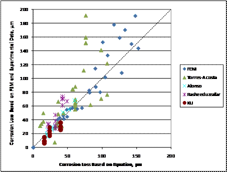
Figure 266. Graph. Corrosion loss in localized corrosion specimens versus corrosion loss predicted by the equation in figure 263 and figure 264 for three-dimensional finite element model and experimental data.
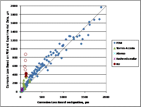
Figure 267. Graph. Corrosion loss in localized corrosion specimens versus corrosion loss predicted by the equation in figure 263 and figure 264 for three-dimensional finite element model and experimental data (revised scale).
Figure 266 covers the range of the experimental data in table 68. There is a moderate degree of scatter for both the finite element model and experimental results, but the finite element model generally agrees with the experimental data. The equations in figure 263 and figure 264 provide a generally conservative estimate of the corrosion loss required to crack concrete based on both the experimental and finite element results; that is, in most cases, the equations in figure 263 and figure 264 underestimate the loss required to cause a crack to form.
The finite element models extend well beyond the range of
experimental data (see figure 267); additional testing will be needed to verify
the accuracy of the finite element model in this range. The KU specimens with actual corrosion losses between 350 and 900 ![]() m (14 and 35
mil) represent the epoxy-coated bars with half-rings and holes in the
epoxy. Figure 263 and figure 264 are very conservative
for these specimens, predicting losses of approximately 200
m (14 and 35
mil) represent the epoxy-coated bars with half-rings and holes in the
epoxy. Figure 263 and figure 264 are very conservative
for these specimens, predicting losses of approximately 200 ![]() m (7.8 mil),
compared to the 350 and 900
m (7.8 mil),
compared to the 350 and 900 ![]() m (14 and 35
mil) range in actual losses. The equation is most conservative for the
epoxy-coated specimens with two holes in the epoxy; these specimens are shown
as open circles in figure 267, as the uncertainty in the exposed area due to
blistering of the epoxy calls the accuracy of these data points into question.
m (14 and 35
mil) range in actual losses. The equation is most conservative for the
epoxy-coated specimens with two holes in the epoxy; these specimens are shown
as open circles in figure 267, as the uncertainty in the exposed area due to
blistering of the epoxy calls the accuracy of these data points into question.
Torres-Acosta and Sagues derived an expression, shown in figure 268, relating bar cover, bar diameter, and localized corrosion length with the corrosion loss required for crack initiation based on experimental results.(71)
![]()
Figure 268. Equation. Torres-Acosta and Sagues' corrosion loss to crack initiation.
Where:
xcrit = Corrosion
loss at crack initiation, ![]() m.
m.
C = Cover, mm.
D = Bar diameter, mm.
L= Length of exposed steel, mm.
Figure 269 and figure 270 compare the corrosion losses predicted by the equation with the experimental data for localized corrosion of ECR presented in table 62, as well as the finite element results and the experimental results presented by Rasheeduzzafar et al., Alonso et al., and Torres-Acosta and Sagues, as done for the equations in figure 263 and figure 264 in figure 266 and figure 267.(68,69,71)
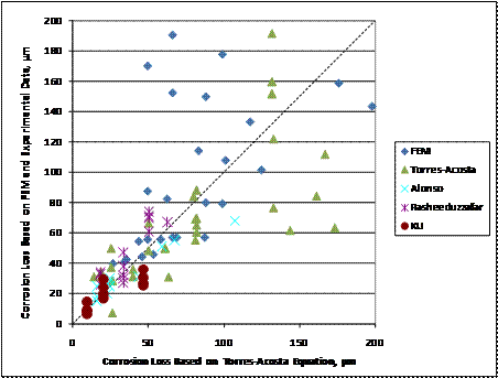
Figure 269. Graph. Corrosion loss in localized corrosion specimens versus corrosion loss predicted by the equation in figure 268 with three-dimensional finite element model and experimental data.
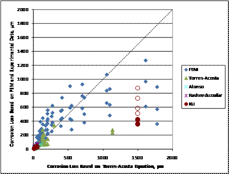
Figure 270. Graph. Corrosion loss in localized corrosion specimens versus corrosion loss predicted by the equation in figure 268 with three-dimensional finite element model and experimental data (revised scale).
Comparing figure 266 and figure 269 shows that for bars that
require less than 50 ![]() m (2 mil) of loss to crack
concrete, the equations in figure 263 and figure 264 and the equation in figure
268 perform comparably. However, the equation
developed by Torres-Acosta is less conservative based on both experimental and
finite element model results for bars that require greater than 50
m (2 mil) of loss to crack
concrete, the equations in figure 263 and figure 264 and the equation in figure
268 perform comparably. However, the equation
developed by Torres-Acosta is less conservative based on both experimental and
finite element model results for bars that require greater than 50 ![]() m (2 mil) of
loss to crack concrete; that is, the corrosion loss required to crack concrete predicted by the equation in figure 268 is greater
than the corrosion loss required to crack concrete in the test specimens
and for many of the finite element results. The equations in figure 263 and figure 264, in contrast, are more conservative
with respect to many of the experimental specimens. The equation in figure 268 overestimates a
significant portion of the experimental results obtained by Torres-Acosta
and Sagues, in one case predicting a corrosion loss of 173
m (2 mil) of
loss to crack concrete; that is, the corrosion loss required to crack concrete predicted by the equation in figure 268 is greater
than the corrosion loss required to crack concrete in the test specimens
and for many of the finite element results. The equations in figure 263 and figure 264, in contrast, are more conservative
with respect to many of the experimental specimens. The equation in figure 268 overestimates a
significant portion of the experimental results obtained by Torres-Acosta
and Sagues, in one case predicting a corrosion loss of 173 ![]() m (6.81 mil) for
a specimen that only required 63
m (6.81 mil) for
a specimen that only required 63 ![]() m (2.48 mil) of loss to crack
concrete. For all experimental specimens
with actual losses greater than 60
m (2.48 mil) of loss to crack
concrete. For all experimental specimens
with actual losses greater than 60 ![]() m (2.4 mil), the equation in figure
268 overestimates the corrosion loss
requited to crack concrete for over 75 percent of the specimens. In comparison,
the equation in figure 263 and figure 264 overestimates the corrosion loss to
crack concrete for only 14 percent of the specimens with actual losses greater
than 60
m (2.4 mil), the equation in figure
268 overestimates the corrosion loss
requited to crack concrete for over 75 percent of the specimens. In comparison,
the equation in figure 263 and figure 264 overestimates the corrosion loss to
crack concrete for only 14 percent of the specimens with actual losses greater
than 60 ![]() m
(2.4 mil).
m
(2.4 mil).
Comparing the two expressions based on results from the finite
element model suggests that the equation in figure 268 becomes increasingly
inaccurate and unconservative for bars that require very large corrosion losses
to crack concrete (see figure 270). Furthermore, results from the finite
element models where greater than 1,200 ![]() m (47 mil) of loss is required
to crack concrete do not appear in figure 270, as the equation in figure 268
predicts that greater than 2,000
m (47 mil) of loss is required
to crack concrete do not appear in figure 270, as the equation in figure 268
predicts that greater than 2,000 ![]() m (79 mil) of loss is
required to crack the concrete.
m (79 mil) of loss is
required to crack the concrete.
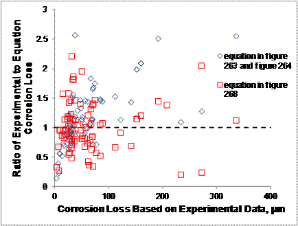
The ratio of experimentally obtained corrosion losses
required to crack concrete to the corrosion losses
obtained by the two equations is also used to judge the degree of conservatism
in each equation. A ratio less than 1.0 indicates an unconservative
estimate for that specimen. Figure 271 and figure
272 compare this ratio for each equation based on corrosion losses obtained
from experimental and finite element
model results, respectively. Over the range of available experimental data, the two equations perform comparably, with the
equations in figure 263 and figure 264 being more conservative for systems where actual losses exceeded 50 ![]() m (2 mil).
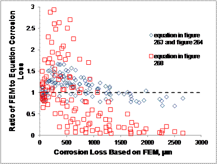
As previously discussed, the
available experimental data involves exposed areas far larger than those
typically observed on damaged ECR. The specimens with damaged ECR tested
as part of this study developed blisters that greatly increased the exposed
area; therefore, only finite element model results are available for small
exposed areas. Over the range of finite element model data, the equation in figure
268 rapidly becomes unconservative, as noted by the large percentage of ratios
of finite element model-predicted corrosion losses to figure 268-predicted
losses that are much less than 1.0 for models with expected corrosion losses
greater than 500
m (2 mil).
As previously discussed, the
available experimental data involves exposed areas far larger than those
typically observed on damaged ECR. The specimens with damaged ECR tested
as part of this study developed blisters that greatly increased the exposed
area; therefore, only finite element model results are available for small
exposed areas. Over the range of finite element model data, the equation in figure
268 rapidly becomes unconservative, as noted by the large percentage of ratios
of finite element model-predicted corrosion losses to figure 268-predicted
losses that are much less than 1.0 for models with expected corrosion losses
greater than 500 ![]() m (20 mil). In contrast, the
equations in figure 263 and figure 264 do not exhibit this behavior. Therefore,
the equations in figure 263 and figure 264 are used to determine the corrosion
loss required to crack concrete for damaged ECR.
m (20 mil). In contrast, the
equations in figure 263 and figure 264 do not exhibit this behavior. Therefore,
the equations in figure 263 and figure 264 are used to determine the corrosion
loss required to crack concrete for damaged ECR.
1 ![]() m = 0.0394 mil
m = 0.0394 mil
Figure 271. Graph. Ratio of experimentally derived corrosion loss to predicted corrosion loss versus corrosion loss to crack concrete based on experimental data.
1 ![]() m = 0.0394 mil
m = 0.0394 mil
Figure 272. Graph. Ratio of finite element model-derived corrosion loss to predicted corrosion loss versus corrosion loss to crack concrete based on finite element model.