U.S. Department of Transportation
Federal Highway Administration
1200 New Jersey Avenue, SE
Washington, DC 20590
202-366-4000
Federal Highway Administration Research and Technology
Coordinating, Developing, and Delivering Highway Transportation Innovations
| REPORT |
| This report is an archived publication and may contain dated technical, contact, and link information |
| Publication Number: FHWA-HRT-12-022 Date: May 2012 |
Publication Number: FHWA-HRT-12-022 Date: May 2012 |
The pier scour formulation developed in this study was tested using laboratory and field data. First, a comparison between the various equation forms indicating maximum potential scour and the data is presented. Then, a specific comparison of the data and the proposed scour equation form is provided.
The equation for maximum scour derived from the framework proposed in this study and represented in figure 50 may be compared with equations for maximum scour from Laursen (figure 3), CSU (figure 4 with K1 = K2 = K4 =1, K3 =1.1, and F = 0.8), and Sheppard-Melville (figure 12). The laboratory and field data are shown in figure 59. The figure shows that the proposed framework indicates the lowest normalized scour, ys/b, for h/b is less than 6, while the Sheppard-Melville equation indicates the lowest normalized scour for h/b is greater than 6. These two relationships provide an envelope for the observed laboratory and field data. The other equations appear to be unnecessarily conservative. The data presented do not contain an observation for normalized scour greater than 2.0. As reported by Ettema et al., 2.5 is the maximum normalized scour.(3)
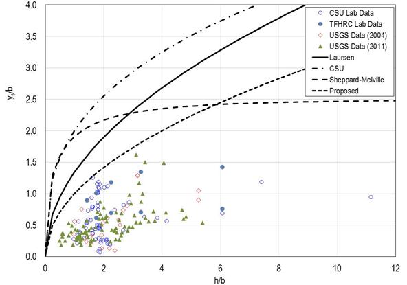
Figure 59. Graph. Comparison of equations for maximum potential scour.
This research suggests that the equation in figure 50 may be used for rough design when h/b is less than 6, and a constant value of 2.5 may be used when h/b is greater than 6 (deep water or narrow piers). This simple framework may also be useful to bridge managers during flood events. Bridge managers could estimate scour conditions at critical moments and formulate timely corrective strategies. A bridge may be considered at less risk if the estimated scour depth, ys, is less than the foundation depth. Otherwise, the bridge may be at greater (or critical) risk and should be closed for public safety. Any damage should be immediately repaired after the flood event.
As indicated by the data in figure 59, the equation in figure 50 is likely overly conservative for many design situations. Therefore, further assessment of the more comprehensive equation in figure 46 was conducted. The laboratory and field data are plotted in figure 60 along with the equation in figure 46 using values of Hcp equal to 0.0, 0.6, 0.9, and 1.2. Most laboratory data fall into a narrow band between the curves for Hcp = 0.0 and Hcp = 1.2. However, much of the field data are above the curves, suggesting that the general form using the hyperbolic tangent formulation is reasonable but could be improved.
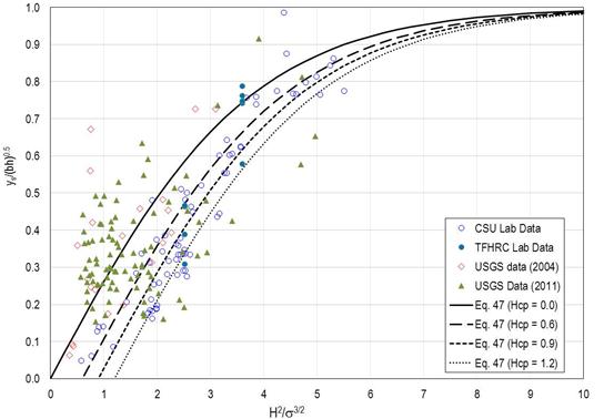
Figure 60. Graph. Confirmation of equation form.
The scatter of data in figure 60 results from the fact that a universal critical value of H2/σ3/2 does not exist for pier scour inception but varies with the flow-structure-sediment conditions, according to Hager and Oliveto.(18) In addition, estimation of Hcp for purposes of accurate scour predictions has not been confirmed. To eliminate uncertainties in estimating Hcp and to develop a conservative design equation, the Hcp parameter is dropped from the equation in figure 46, leaving the equation in figure 61.
![]()
Figure 61. Equation. Initial design equation.
Although a conservative design equation is advantageous, it is undesirable to be unnecessarily conservative. To address this, several of the parameters in the equation in figure 61 were optimized considering the laboratory and field data. The equation in figure 62 illustrates the parameters that were optimized.

Figure 62. Equation. Design equation showing optimized parameters.
The parameters for A, B, C, D, and λ were determined as shown in the final design equation in figure 63.
![]()
Figure 63. Equation. Final design equation.
Using the laboratory data and USGS field data, the relative scour, ys/(b0.62 × h0.38), computed from the final design equation is compared to the measured relative scour depth in figure 64. Of the 190 measured values, 181 were overpredicted, and 9 were underpredicted. Of the overpredicted values, the root mean square (RMS) error was 0.44.
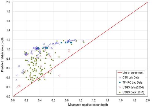
Figure 64. Graph. Predicted versus measured relative scour: proposed equation.
The same comparisons were performed using the CSU equation and the Sheppard-Melville equation and are shown in figure 65 and figure 66, respectively. (Critical velocity for the Sheppard-Melville equation was computed using the equation in figure 11.)
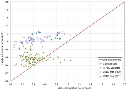
Figure 65. Graph. Predicted versus measured relative scour: CSU equation.
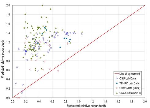
Figure 66. Graph. Predicted versus measured relative scour: Sheppard-Melville equation.
Table 5 provides a summary of the evaluation measures for the proposed design equation and the CSU and Sheppard-Melville equations. The proposed equation is comparable in the number and percent of predictions that are conservative compared with the other two methods. It performs slightly better than the CSU equation and significantly better than the Sheppard-Melville equation in terms of reducing the overprediction, as measured in the RMS error.
Table 5 also provides a reliability index (RI) that measures the risk of underpredicting the actual value. A higher RI indicates a lower risk of underprediction. It is calculated as (RI) = (1–Mx)/Sx where Mx is the mean and Sx is the standard deviation of a series of x values. In this case, x is defined as the ratio of the measured scour to the predicted scour. The risk of underpredicting is lowest with the Sheppard-Melville equation and greatest with the CSU equation.
Compared with the CSU equation, the proposed equation has a lower RMS error and higher RI, indicating that the proposed equation would be an improvement over the CSU equation. Therefore, the proposed equation, formulated based on the sediment-structure-flow interactions, is recommended for use.
Table 5. Comparison of design equations.
| Equation | Number Conservative | Percent Conservative | RMS Error for Conservative Predictions | RI |
|---|---|---|---|---|
| Proposed | 181 | 95.3 | 0.44 | 1.85 |
| CSU | 176 | 92.6 | 0.46 | 1.33 |
| Sheppard-Melville | 184 | 96.8 | 0.82 | 3.23 |
The proposed equation in figure 63 is for a simple cylindrical pier. Although no new analyses were conducted as part of this study, the correction factors from HEC-18 for pier nose shape, angle of attack, and bed condition are considered applicable.(2) Therefore, the equation including these factors is presented in figure 67.

Figure 67. Equation. Final design equation with correction factors.
The recommended pier scour design equation was developed by considering scour processes as they are driven by flow, structure, and sediment interactions. It was refined by comparing predicted to measured scour and attempting to minimize the extent of overprediction while remaining conservative, as is appropriate for design.
This equation is most appropriately applied to the following conditions represented in the data used for evaluating the equation:
Since the equation form was developed from an evaluation of general processes, these ranges should not be considered strict limits but, rather, representative conditions. The designer must consider the applicability of this equation outside these conditions on a site-specific basis.