U.S. Department of Transportation
Federal Highway Administration
1200 New Jersey Avenue, SE
Washington, DC 20590
202-366-4000


Skip to content
Facebook iconYouTube iconTwitter iconFlickr iconLinkedInInstagram

Federal Highway Administration Research and Technology
Coordinating, Developing, and Delivering Highway Transportation Innovations

 
REPORT
This report is an archived publication and may contain dated technical, contact, and link information
Back to Publication List        
Publication Number:  FHWA-HRT-14-087    Date:  March 2015
Publication Number: FHWA-HRT-14-087
Date: March 2015


Computer-Based Guidelines for Concrete Pavements, HIPERPAV III, Version 3.3 User's Manual

Chapter 5. Reports

For any HIPERPAV III® version 3.3 analysis, reports can be generated by clicking the print icon in the upper icon toolbar or by selecting "Print" from the file menu. After selecting "Print" a HIPERPAV® Report window is displayed as shown in figure 69. In this window, icons in the top left allow the user to print the report as shown, preview the report, and export the results to a Microsoft® Excel spreadsheet.
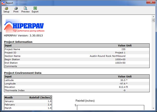
Figure 69. Screen Capture. HIPERPAV report window. This image shows the top half of a HIPERPAV report. The HIPERPAV® logo and version number appear in the top left corner. Data shown are grouped in boxes under the following headings: Project Information and Project Environment Data. Input categories and values are listed.

Figure 69. Screen Capture. HIPERPAV® Report window.

COMET Module

The Concrete Optimization, Management, Engineering, and Testing (COMET) module is a simplified derivation of the Concrete Optimization Software Tool that was developed by FHWA and the National Institute of Standards and Technology for optimizing concrete mixes. COMET can be accessed within HIPERPAV® by selecting "COMET" in the tools drop-down menu in the main toolbar, shown in figure 70. COMET optimizes concrete mixes based on early-age strength, 28-day strength, and cost.
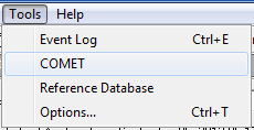
Figure 70. Screen Capture. Tools drop-down menu in HIPERPAV®. Tools and Help appear at the top of the image. The options listed in the drop-down menu under Tools are shown. The options are Event Log, COMET, Reference Database, and Options. COMET is highlighted.

Figure 70. Screen Capture. Tools drop-down menu in HIPERPAV®.

Once selected, the initial COMET window appears as shown in figure 71. Inputs and outputs can be selected from the menu-like list on the left side of the window. The inputs for the window selected are displayed on the right. The first item on the tree view, "Event Log", reports potential problems that may arise while running the software. Also, the tree view shows two levels of inputs and outputs. Level 1 inputs generate the experiment design of trial batches required for optimization. Level 2 inputs produce a set of optimum mixes based on the trial batch test results, and desirability functions defined for each response (early-age strength, 28-day strength, and cost).

As shown in figure 71, mix constituents are limited to cement, pozzolan, water, coarse aggregate, and fine aggregate. For each constituent, the specific gravity and cost is required.
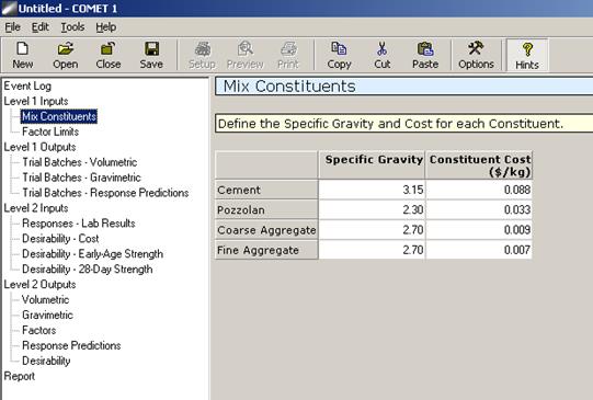
Figure 71. Screen Capture. Mix Constituents input window in COMET. The Mix Constituents input window is shown with an Event Log table of contents listed that appears to the left of the input window. Mix Constituents is highlighted in the log under Level 1 Inputs. A note appears at the top of the Mix Constituents window that reads as follows: Define the Specific Gravity and Cost for each Constituent. Beneath the note is a table with three columns and five rows. The cells in the first column have the following headings: Cement, Pozzolan, Coarse Aggregate, and Fine Aggregate. The first row for columns two and three has the headings: Specific Gravity and Constituent Cost (in dollars per kilogram). All other cells include example data.

Figure 71. Screen Capture. Mix Constituents input window in COMET.

The user provides optimization ranges for coarse aggregate fraction, cementitious content, pozzolan substitution, and water-to-cement (w/cm) ratio (see figure 72).
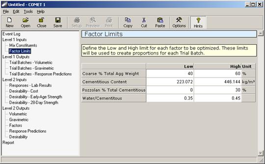
Figure 72. Screen Capture. Factor Limits input window in COMET. The Factor Limits input window is shown with an Event Log table of contents listed that appears to the left of the input window. Factor Limits is highlighted in the log under Level 1 Inputs. A note appears at the top of the Factor Limits input window that prompts the user to define limits for optimizing factors and alerts the user that these limits will be used to create proportions for trial batches. Beneath the note is a table with four columns and five rows. The cells in the first column and first row have the following headings: Coarse % Total Agg Weight, Cementitious Content, Pozzolan % Total Cementitious, and Water/Cementitious. The first row for columns two, three, and four has the headings: Low, High, and Unit. All other cells include example data.

Figure 72. Screen Capture. Factor Limits input window in COMET.

With the inputs in Level 1, trial batches are developed for the experimental program by running the "Create Trial Batches" command button in the Level 1 outputs window, as shown in
figure 73. As a result, 29 trial batches are generated, which can be displayed in volumetric (percent of total volume) and gravimetric (weight per unit of volume) form. The gravimetric form is presented in figure 74.
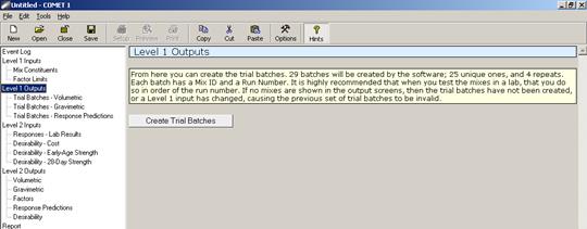
Figure 73. Screen Capture. Create trial batches command button in Level 1 Outputs. The Level 1 Outputs window is shown with an Event Log table of contents listed that appears to the left of the output window. Level 1 Outputs is highlighted in the log. A note appears at the top of the Level 1 Outputs window that reads as follows: From here you can create the trial batches. 29 batches will be created by the software; 25 unique ones, and 4 repeats. Each batch has a Mix ID and a Run Number. It is highly recommended that when you test the mixes in a lab, that you do so in order of the run number. If no mixes are shown in the output screens, then the trial batches have not been created, or a Level 1 input has changed, causing the previous set of trial batches to be invalid. Beneath the note is an icon labeled Create Trial Batches.
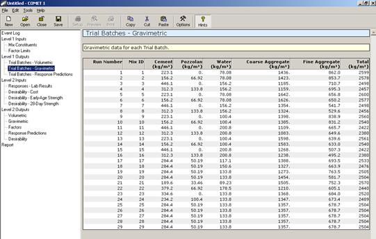
Figure 73. Screen Capture. Create trial batches command button in Level 1 Outputs.

Figure 74. Screen Capture. Trial batches in kg/m3, gravimetric form. The Trial Batches—Gravimetric output window is shown with an Event Log table of contents listed that appears to the left of the output window. Trial Batches—Gravimetric is highlighted in the log under Level 1 Outputs. A note appears at the top of the Trial Batches—Gravimetric input window that states the following: Gravimetric data for each Trial Batch. Below the note is a table with 8 columns and 30 rows. Column headings appear in the first row and are Run Number, Mix ID, Cement (kg/m3), Pozzolan (kg/m3), Water (kg/m3), Coarse Aggregate (kg/m3), Fine Aggregate (kg/m3), and Total (kg/m3). Respective data for 29 mixes appear in the cells of the remaining rows.

Figure 74. Screen Capture. Trial batches in kg/m3, gravimetric form.

In addition, as shown in figure 75, the cost for every trial batch is computed, and default models in COMET are used to predict early-age strength and 28-day strength as a function of mix constituents. Predicted responses are only approximate and may be used in a planning stage in which the mix constituents may not be known or are not available for testing.
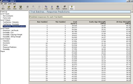
Figure 75. Screen Capture. Predicted responses for each trial batch. The Trial Batches—Response Predictions output window is shown with an Event Log table of contents listed that appears to the left of the output window. Trial Batches—Response Predictions is highlighted in the log under Level 1 Outputs. A note appears at the top of the Trial Batches—Response Predictions output window that states the following: Predicted Responses for each Trial Batch. Below the note is a table with 5 columns and 30 rows. Column headings appear in the first row and are Run Number, Mix Number, Cost (dollars per cubic meter), Early-Age Strength (MPa), and 28-Day Strength (MPa). Respective data for 29 mixes appear in the cells of the remaining rows.

Figure 75. Screen Capture. Predicted responses for each trial batch.

After the Level 1 inputs and outputs are complete, the user can proceed with Level 2 analysis. To continue with this analysis, the user must enter the laboratory testing results for each response for the trial batches generated in Level 1 (see figure 76). Alternatively, the user may fill in these values using default models by clicking the "Reset to Predicted Values" command button, if a preliminary analysis is desirable.
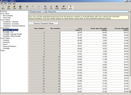
Figure 76. Screen Capture. Lab results window. The Responses—Lab Results input window is shown with an Event Log table of contents listed that appears to the left of the input window. Responses—Lab Results is highlighted in the log under Level 2 Inputs. A note appears at the top of the Responses—Lab Results input window that states the following: You can use the predicted responses from the previous section or override them with your values from lab tests (recommended). Click the 'Reset' button to reset these values back to the predicted response values. Below the note is a table with 5 columns and 24 rows. Column headings appear in the first row and are Run Number, Mix Number, Cost (dollars per cubic meter ), Early-Age Strength (MPa), and 28-Day Strength (MPa). Respective data for 23 mixes appear in the cells of the remaining rows.

Figure 76. Screen Capture. Lab results window.

The user can assign desirability functions for each of the optimization responses under the cost, early-age strength, and 28-day strength desirability windows. (A sample desirability function is shown in figure 77 for 28-day strength.)
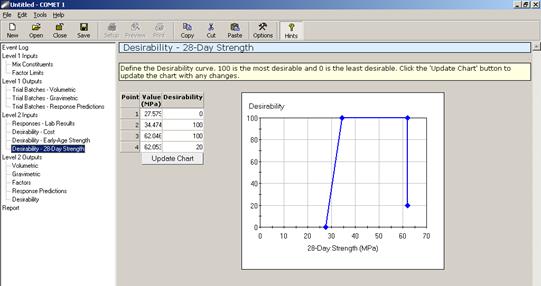
Figure 77. Screen Capture. Desirability function for 28-day strength. Desirability—28-Day Strength input window is shown with an Event Log table of contents listed that appears to the left of the input window. Desirability—28-Day Strength is highlighted in the log under Level 2 Inputs. A note appears at the top of the Responses—Lab Results input window that states the following: Define the Desirability curve. 100 is the most desirable and 0 is the least desirable. Click the 'Update Chart' button to update the chart with any changes. Below the note is a table with three columns and five rows. Column headings appear in the first row and are Point, Value (MPa), and Desirability. Example data populate the active cells. Below the chart is an icon labeled Update Chart. To the right of the table is a chart titled Desirability. 28-Day strength (MPa) is shown on the x-axis with values from 0 to 70. The y-axis values range from 0 to 100.

Figure 77. Screen Capture. Desirability function for 28-day strength.

After the Level 2 inputs are entered, optimization of mixes is performed by clicking the "Optimize Mixes" command button in the Level 2 outputs window (see figure 78). With this command, regression models based on the results from the experimental program or from the predicted responses are developed as a function of the mix proportions.
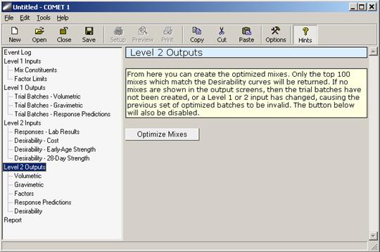
Figure 78. Screen Capture. Level 2 outputs—command to optimize mixes. The Level 2 Outputs window is shown with an Event Log table of contents listed that appears to the left of the output window. Level 2 Outputs is highlighted in the log. A note appears at the top of the Level 2 Outputs window that reads as follows: From here you can create the optimized mixes. Only the top 100 mixes which match the Desirability curves will be returned. If no mixes are shown in the output screens, then the trial batches have not been created, or a Level 1 or 2 input has changed, causing the previous set of optimized batches to be invalid. The button below will also be disabled. Beneath the note is an icon labeled: Optimize Mixes.

Figure 78. Screen Capture. Level 2 outputs-command to optimize mixes.

These models predict responses for a comprehensive set of mixtures within the factor limits specified in the factor limits window. Finally, optimum mixes are identified in terms of the individual desirability for every response and the maximum overall desirability for all responses, and are presented in volumetric and gravimetric form. Optimum mixes are shown in volumetric form in figure 79.
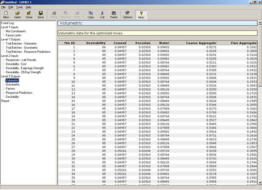
Figure 79. Screen Capture. Optimum mixes sorted by desirability in volumetric form. The Volumetric output window is shown with an Event Log table of contents listed that appears to the left of the output window. Volumetric is highlighted in the log under Level 2 Outputs. A note appears at the top of the Volumetric output window that reads as follows: Volumetric data for the optimized mixes. Below the note is a table with 7 columns and 36 rows of data showing. There is a scroll bar along the far right side of the window. Column headings appear in the first row and are Mix ID, Desirability, Cement, Pozzolan, Water, Coarse Aggregate, and Fine Aggregate. Respective data for 35 mixes appear in the cells of the remaining rows.

Figure 79. Screen Capture. Optimum mixes sorted by desirability in volumetric form.

In addition, the optimum mixes are also displayed in terms of the optimization factors, predicted responses, and individual response desirabilities as shown in figure 80, figure 81, and figure 82 respectively.
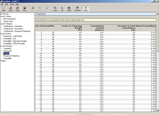
Figure 80. Screen Capture. Optimum mixtures in terms of optimization factors. The Factors output window is shown with an Event Log table of contents listed that appears to the left of the output window. Factors is highlighted in the log under Level 2 Outputs. A note appears at the top of the Factors output window that reads as follows: Calculated mix proportions for each optimized mix. Below the note is a table with 7 columns and 36 rows of data showing. There is a scroll bar along the far right side of the window. Column headings appear in the first row and are Mix ID, Desirability, Cement, Pozzolan, Water, Coarse Aggregate, and Fine Aggregate. Respective data for 35 mixes appear in the cells of the remaining rows.
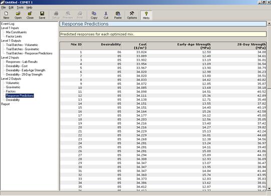
Figure 80. Screen Capture. Optimum mixtures in terms of optimization factors.

Figure 82. Screen Capture. Individual response desirability’s for optimum mixtures. The Desirability output window is shown with an Event Log table of contents listed that appears to the left of the output window. Desirability is highlighted in the log under Level 2 Outputs. A note appears at the top of the Desirability output window that reads as follows: Predicted response desirability values for each optimized mix. Below the note is a table with 5 columns and 37 rows of data showing. There is a scroll bar along the far right side of the window. Column headings appear in the first row and are Mix ID, Desirability, Cost, Early-Age Strength, 28-Day Strength. Respective data for 36 mixes appear in the cells of the remaining rows.

Figure 81. Screen Capture. Response predictions for optimum mixtures.
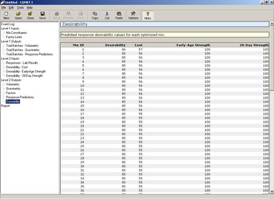
Figure 81. Screen Capture. Response predictions for optimum mixtures.The Response Predictions output window is shown with an Event Log table of contents listed that appears to the left of the output window. Response Predictions is highlighted in the log under Level 2 Outputs. A note appears at the top of the Response Predictions output window that reads as follows: Predicted responses for each optimized mix. Below the note is a table with 7 columns and 36 rows of data showing. There is a scroll bar along the far right side of the window. Column headings appear in the first row and include Mix ID, Desirability, Cement, Pozzolan, Water, Coarse Aggregate, and Fine Aggregate. Respective data for 35 mixes appear in the cells of the remaining rows.

Figure 82. Screen Capture. Individual response desirabilities for optimum mixtures.

A report that can be used for printing the inputs and outputs for the entire analysis is generated, as shown in figure 83. To print, click on the print icon on the upper icon toolbar.
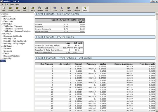
Figure 83. Screen Capture. Report view for printing purposes. The report output window is shown to the right of an Event Log table of contents, where Report is highlighted. The first section of the report has the heading Level 1 Inputs: Mix Constituents. A table includes columns showing Specific Gravity and Constituent Cost in dollars per kilogram. Each row lists a constituent and shows sample data in both columns. The second section of the report has the heading Level 1 Inputs: Factor Limits. A table includes columns showing Low, High, and Unit. Each row lists a factor, including Coarse % Total Agg Weight, Cementitious Content, Pozzolan % Total Cementitious, and Water/Cementitious. Sample data is shown in the three columns. The third section of the report has the heading Level 1 Outputs: Trial Batches—Volumetric. A table includes columns showing Run Number, Mix Number, Cement, Pozzolan, Water, Coarse Aggregate, and Fine Aggregate. Run and mix numbers begin at 1 and increase by 1 in the following rows. Sample data are shown in the remaining columns.

Figure 83. Screen Capture. Report view for printing purposes.

REFERENCES

  1. Ruiz, J.M., Rasmussen, R.O., Chang, G.K., Dick, J.C., and Nelson, P.K. Computer-Based Guidelines for Concrete Pavements Volume II-Design and Construction Guidelines and HIPERPAV II® User's Manual, Office of Infrastructure Research and Development, FHWA-HRT-04-122, Federal Highway Administration, February 2005.
  2. Ruiz, J.M., Xu, Q., Chang, G.K., Dick, J.C., Garber, S.I., and Rasmussen R.O. HIPERPAV III® Moisture Transport and Sensitivity Analysis Enhancements, FHWA-09-048, Federal Highway Administration, January 2009.
  3. Ioannides, A.M. and Korovesis, G.T., "Analysis and Design of Doweled Slab-on-Grade Pavement Systems," Journal of Transportation Engineering, 118(6), pp. 745-768, November-December 1992.
  4. Robert, O.R. and Rozycki, D.K., "Characterization and Modeling of Axial Slab-Support Restraint," Transportation Research Record No. 1778, Transportation Research Board, National Research Council, Washington, DC, 2001.
  5. FHWA. Coefficient of Thermal Expansion in Concrete Pavements, Advanced Concrete Pavement Technology Program, FHWA-HIF-09-015, Washington, DC, October 2011.


Federal Highway Administration | 1200 New Jersey Avenue, SE | Washington, DC 20590 | 202-366-4000
Turner-Fairbank Highway Research Center | 6300 Georgetown Pike | McLean, VA | 22101