U.S. Department of Transportation
Federal Highway Administration
1200 New Jersey Avenue, SE
Washington, DC 20590
202-366-4000
Federal Highway Administration Research and Technology
Coordinating, Developing, and Delivering Highway Transportation Innovations
| REPORT |
| This report is an archived publication and may contain dated technical, contact, and link information |
|
| Publication Number: FHWA-HRT-07-040 Date: October 2011 |
Publication Number: FHWA-HRT-07-040 Date: October 2011 |
A primary goal of the updated calibration protocol is universal compatibility with the four brands of FWDs used in North America. Interviews conducted with the FWD manufacturers, calibration operators, some owners, and other FWD experts determined what problems were encountered during calibration with the old SHRP procedure. The following sections discuss calibration of the four brands of FWDs as well as known issues associated with their calibration.
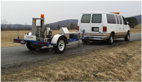
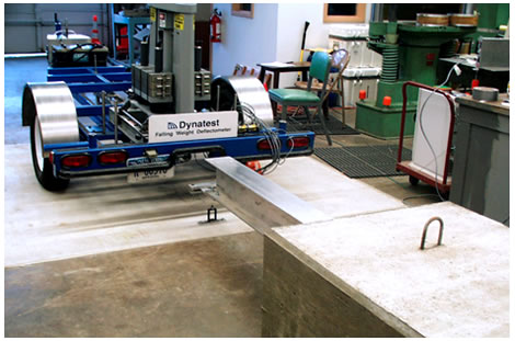
The first Dynatest® FWD was manufactured in Denmark in 1976, and the first one was sent to the United States in 1981.(13) Dynatest® manufactures two varieties of FWDs, the model 8000 FWD and the model 8081 HWD. Both systems are trailer-mounted with 11.7-inch (300-mm) loading plates (with an optional 17.55-inch (450-mm) plate available) and can have between
Figure 6. Photo. Dynatest® model 8000 trailer-mounted FWD.
Dynatest® FWDs consist of a hydraulically controlled single-mass system. Weights can be removed or added to change the magnitude of the load pulse. The standard equipment places one deflection sensor directly under the load plate, and at least six additional deflection sensors are placed along a raise-lower bar. The geophone sensor bar runs from the load plate toward the tow vehicle. Additional deflection sensors can be positioned on a rear or transverse extension bar. The deflection sensors are velocity transducers (geophones), and the deflections are calculated using a single integration of the velocity response.
The HWD normal load levels exceed the usual 6,000-, 9,000-, 12,000-, and 16,000-lbf (27-, 40-, 53-, and 71-kN) range specified in the original SHRP calibration procedure. In order for the HWD to achieve the preferred load levels, all attached weights must be removed. This causes some concern about whether the calibration is valid for the HWD since it is not normally used with all weights removed.
However, both load and deflection calibration procedures under the old and the new protocols have very tight tolerance requirements for sensor linearity. This assures that the sensors are performing linearly over the calibration range.
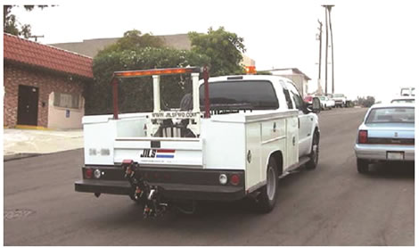
The first JILS FWD was made in 1987 in the United States.(14) JILS manufactures the following four varieties of FWDs:
All JILS FWDs use a 12-inch (305-mm) rigid steel loading plate and have an optional 12-inch (305-mm) segmented or 18-inch (457-mm) rigid loading plate. The deflection sensors are velocity transducers, and their response is single-integrated to determine the deflection. A unique feature of a JILS FWD is its ability to report both the first and second peaks of each drop. The second peak is not calibrated in the AASHTO R32-09 procedure.(1)
Previously, the lack of a swivel on the load plate has made calibration difficult in some locations (although the manufacturer has recently announced that a swivel is now an available option). Without a swivel, the calibration operator must ensure that the load plate is squarely seated on the reference load cell without any gaps around the perimeter. Since the standard JILS load plate is slightly larger than the 11.7-inch (300-mm) diameter of the reference load cell, adjustments have been made to the original design of the reference load cell. The guide fingers have also been adjusted to accommodate the JILS load plate.
Two additional issues posed challenges for calibrating JILS using the SHRP procedure. The machine uses a large mass with a short drop height. As a result, it was difficult to achieve optimal triggering at the low drop height due to the short free fall time as well as mechanical vibration. Additionally, JILS applies a large static preload on the pavement. This frequently causes clipping of the load response at the high drop height. These problems have been reduced in the new AASHTO R32-09 procedure.(1)
Figure 7. Photo. JILS-20T truck-mounted FWD.
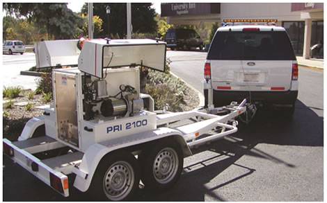
Carl Bro manufactures both a double-axle trailer-mounted FWD and a vehicle-mounted FWD.(15) The two loading plate options are a four-segmented 11.7-inch (300-mm)-diameter plate or a 17.55-inch (450-mm) plate. A single mass is used and controlled hydraulically. The minimum number of deflection sensors is 9, and the maximum is 18. One sensor is used to measure deflection through the center of the load plate, while the remaining sensors can be placed on the raise-lower bar oriented toward the tow vehicle or on the side or rear using a T-beam. The deflection sensors are velocity transducers, and their response is single integrated to determine the deflection. Figure 8 shows an example of a Carl Bro FWD.
Figure 8. Photo. Carl Bro FWD.
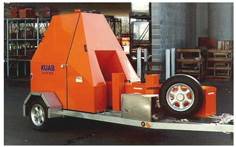
KUAB has been manufacturing FWDs since 1976, and the first one was sent to the United States in 1988.(14) KUAB manufactures both trailer-mounted and vehicle-mounted FWDs that are either single- or dual-mass. Most KUAB FWDs use seismometers to measure deflections. Velocity transducers (geophones) are available as an option for some models. The overall number of deflection sensors is unlimited according to the specification, although the KUAB-50 model has seven sensors. The sensors can be aligned either toward the tow vehicle (see figure 9) or away from it. KUAB has the option of either a four-part segmented load plate with an 11.7-inch (300-mm) or 17.55-inch (450-mm) diameter, or it has a rigid load plate with a 5.85-inch (150-mm), 11.7-inch (300-mm), or 17.55-inch (450-mm) diameter. Figure 9 shows a KUAB FWD with geophone sensors.
Figure 9. Photo. KUAB FWD with sensors aligned toward the tow vehicle.
For the KUAB FWD with deflection sensors positioned to the rear of the load plate, positioning the FWD load plate close enough to the LVDT during the SHRP calibration procedure was difficult. This made it hard to trigger the data acquisition system and achieve the desired deflections during geophone reference calibration. About triggering, which is discussed in more detail in a later section, has reduced that issue.
Issues Encountered with the SHRP FWD Calibration Protocol
In addition to the FWD-specific issues cited above, several more general problems were encountered while using the old SHRP procedure and equipment. These included excessive beam movement, difficulty in triggering, and difficulty in getting sufficiently large deflections. Electrical problems included excessive noise in the signal and insufficient power from the battery charger. Also, data acquisition problems affected the speed and accuracy of FWD calibration.
Beam Movement Problems
Beam movement was measured using one of the deflection sensors from the FWD. Figure 10 shows the beam and block combination used in the SHRP protocol. After reference calibration of each deflection sensor, beam movement was determined from the FWD time histories. If beam movement was 0.12 mil (3 μm) or more when the sensor being calibrated peaked out, the calibration was repeated. This problem seemed to be aggravated by water in the soil beneath the test pad, making it a seasonal issue. This forced the FWD owner to return and attempt to calibrate at a later date. It also caused some of the calibration centers to shut down for periods of time (particularly in the spring).
Figure 10. Photo. FWD calibration beam and inertial block.
The SHRP calibration protocol required at least 16 mil (400 μm) of deflection at the 16,000-lbf (71.2-kN) load level during deflection sensor calibration. This meant that the load plate needed to be close to the end of the beam without touching it. Due to geometric constraints, it was difficult to achieve the necessary load plate proximity for several models of FWDs and HWDs.
Data Acquisition Problems
The most common data acquisition problems fell into the following two categories: FWD brand-specific problems and general data problems.
KUAB and JILS FWDs had triggering problems, especially at low load levels. The SHRP procedure used the response of the test pad to trigger the data acquisition system. When the calibration software detected the vibration in the test pad due to the release of the FWD mass, the system began to acquire data. Because of the nature of its mass release system, KUAB FWD did not cause a measurable vibration at the time of release. As a result, the data acquisition system often failed to begin acquiring data. Conversely, JILS produced a lot of vibration when the mass was released, and this often triggered data acquisition too early.
Data transfer from the FWD was a problem with the old SHRP method because while the calibration system software collected and stored data from the reference calibration instrumentation, the data collected from the FWD had to be printed and typed into the calibration system. This increased the probability of transcription errors and took a considerable amount of time.
The software program FWDCAL 4 was written to perform relative calibration data analysis using the SHRP method. Because the program could only read output from older Dynatest® FWDs, a spreadsheet with macros was written to work with additional data formats. However, the spreadsheet did not cover all FWD types and system configurations.
The lack of a common data file format was the main problem. Because each brand of FWD outputs data was in a different native format, calibration operators were required to be experts in reading FWD data. Differences in data file formats occasionally required manual calculations to convert FWD plate pressure to load units. Some but not all of the different brands of FWDs have the ability to directly produce the AASHTO standard PDDX data format.(7) All FWD manufacturers have promised to provide the PDDX output option. Some FWDs use a separate converter program to change their native data format into PDDX format. Unfortunately, the original AASHTO standard format did not provide all of the data needed for FWD calibration.
Other Known Problems
Legislative and financial restrictions limited some State transportation departments from sending people and equipment out of State to one of the FWD calibration centers, preventing them from getting their FWDs calibrated to the SHRP/ LTPP standard. Included in this group were FWDs from other countries such as Canada.
This section discusses the research that led to the development of the new FWD calibration protocol. The detailed procedure is included in appendix A. Specifications for each item of calibration equipment mentioned are provided in appendix E.
The Keithley KUSB-3108 DAQ replaces the Metrabyte model DAS-16G in the new protocol. The Keithley board offers the advantages of USB 2.0 connectivity, which is universally compatible with any computer with USB 1.0 or 2.0 ports and does not require the now obsolete ISA bus.
Initially, the possibility of using an internal peripheral component interconnect (PCI) card was explored. The PCI specification is slowly being phased out in favor of the faster PCI express slot; however, PCI cards are not backwards compatible with the new standard. An external device such as the KUSB-3108 can be easily installed by connecting it to the calibration computer via a standard USB cable. USB standards are backwards compatible and are a common feature of all modern computers.
A feature specific to the chosen model was the availability of drivers compatible with the Microsoft Visual Basic® language in which the WinFWDCal software was written, eliminating the need to develop custom drivers. Keithley supplies a driver set that is compatible with Microsoft Windows XP® and Windows Vista®. The software has been used successfully in both operating systems.
Protection of DAQ Cabling
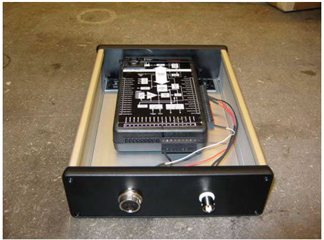
One problem became evident as researchers began using the KUSB-3108 DAQ—the cables are attached to the box via a screw terminal system that leaves the wires vulnerable to being pulled out. Several calibration center operators reported having problems with the wires becoming loose.
An aluminum box was found to be well suited to provide some protection for the wiring (see figure 11). DAQ is held in the box with a strip of Velcro®. Holes are drilled in both ends for connections to the USB port and the input and output channels. The box has a lid, and it can be stored with the lid on. However, the lid should be removed during use so that the DAQ can render an accurate measure of ambient temperature. Details about the box and the related hardware are provided in table 39 of appendix E.
Figure 11. Photo. Box for DAQ wiring protection.
About Triggering
Modern data acquisition equipment allows the use of a technique called "about triggering" to determine when an event has occurred. Using buffers, about triggering allows the collection of data before and after a user-specified threshold value is reached. This means that the data are taken about or around the time when the trigger level is reached. The readings are continuously stored in buffers by WinFWDCal.
Currently, WinFWDCal uses 50 buffers with 300 readings per buffer. Data are collected at a speed of 15,000 readings per second. When each buffer is full, the data in it are scanned to determine if the threshold level (trigger) was exceeded. If it was, the data in the buffer, along with several preceding and following buffers, are saved to create the complete dataset. If not, the oldest data are discarded, and a new set of data is collected and reviewed.
One second of data is saved for analysis: one-third of 1 s before the trigger and two-thirds of 1 s after. With a reading rate of 15,000 Hz, this means 5,000 readings are taken before, and 10,000 readings are taken after the trigger point. This includes data from before the release of the mass to the several bounces after the first main pulse.
Incoming data are read as voltages. Converting the voltages to engineering units requires the sensors (the accelerometer and reference load cell) to be calibrated. The procedures for sensor calibration will be discussed in following sections.
About triggering has streamlined the data-taking process and eliminated the need to have separate hardware to detect the trigger point. It has also eliminated the triggering problem mentioned previously with the KUAB FWD load pulse.
For load calibration, the trigger level must be set high enough to avoid triggering by the preload force but low enough to trigger when the lowest drop level is used. When 10 consecutive readings exceed the trigger level, the about trigger point is set. Using 10 readings eliminates false triggers caused by voltage spikes.
In the case of a Dynatest® or Carl Bro FWD, the preload is about 1,000 lbf (4.5 kN). For a JILS FWD, the preload can be as high as 2,500 lbf (11 kN), while the KUAB preload level is very small. Setting the trigger level at 3,000 or 4,000 lbf (13 or 18 kN) is generally correct for load calibration since the smallest dynamic peak load is usually 6,000 lbf (26 kN).
Setting the appropriate acceleration trigger level requires finding an optimum between the pulse peak from the lowest and highest load levels. Research has shown that this must be tailored for each type of FWD. The pulse durations, and thus, the accelerations, differ from one type of FWD to another. The position of the FWD load plate face-to-face with the accelerometer in the calibration stand is variable. As a result, so are the peak accelerations. The response characteristics of the test pad can also vary from one day to another at the same location, so the trigger level must be determined immediately prior to each FWD calibration.
When the FWD is in place with the accelerometer on the deflection sensor calibration stand, one drop at the low drop height is analyzed to determine an appropriate trigger level for the accelerometer. WinFWDCal performs the analysis.
When the original SHRP FWD reference calibration procedure was developed, the specified drop sequence required five replicate drops at four load levels. Experience with the initial four and later eight Dynatest® FWDs used by SHRP showed that the drop sequence was well suited to check the linearity of the sensors, and 20 drops provided enough data to fit a regression with a good level of confidence.
However, it has been noted that some FWDs had a problem with this drop sequence. For example, JILS uses a heavier mass and a shorter drop distance, and the lowest load level (6,000 lbf (26 kN)), had a much shorter free-fall time than the Dynatest® FWD. Vibration associated with the release of the mass did not have enough time for damping before the mass struck the load plate. Calibration operators reported problems with excess noise messages at the low, and even the second, load level.
This issue was overcome by relying on the experience from performing hundreds of FWD calibrations over the past 15 years. Rather than working with a single fixed drop sequence, researchers were able to allow some flexibility depending on the daily response of the test pad. The solution involves a tradeoff between the number of load levels used and the number of replicate drops required to achieve the desired level of precision.
Either three or four load levels may be used, depending on the preference of the FWD owner or the recommendation of the manufacturer. WinFWDCal determines the required number of replicate drops per load level. The number of drops must be the same at each load level to simplify data collection and analysis. It is also recommend that the same drop sequence be used for both load and deflection sensor calibration.
The goal is for the standard error of the final calibration factors to be no more than 0.003 (i.e., 0.3 percent). Experience with all types of FWDs has shown that the expected random measurement error for one drop is seldom more than ±0.08 mil (±2 μm) deflection and ±20 lbf (±0.09 kN) load. Deflection is the more critical of the two to achieve the desired standard error, so it controls the number of replicate drops.
When the FWD is in place with the accelerometer on the deflection sensor calibration stand, one drop at the low drop height and one at the high drop are analyzed to determine the minimum number of drops needed to achieve the desired precision. WinFWDCal performs the analysis. A total of at least 18 drops is necessary to ensure the minimum statistical power. This requires a minimum of six replicate drops at three load levels or five replicates at four levels.
It was determined that 10 replicate drops per load level were a practical upper limit. If the required number of replicates exceeds 10, the FWD should be repositioned to obtain larger deflections. A larger range of deflections between the lowest and the highest drop height will result in fewer replicate drops needed. Therefore, switching from three to four load levels will usually reduce the required number of drops.
It is important that the drop sequence be determined for each FWD calibration. The routine accounts for the position of the FWD load plate with respect to the sensor stand, and the current properties of the test pad are also factored. The dynamics of the FWD load pulse are considered to reduce the likelihood of excess noise messages. The ability of the software to determine the drop sequence based on the local daily conditions provides flexibility.
As noted in chapter 1, it is important that the peak deflection be sufficiently large to allow a clear distinction between the bias error and the random error. Research has shown that a peak deflection of 20 mil (500 μm) at a force of 16,000 lbf (71 kN) would adequately achieve that goal. Lesser deflections as little as 12 mil (300 μm) may suffice, but the required number of drops increases as peak deflection decreases.
It was found that a test area that is built with a 5-inch (125-mm) fiber-reinforced concrete surface, a 5.85-inch (150-mm) aggregate base, and a 120–200-inch (3–5-m) soft clay subgrade will achieve the target deflection level. The deflection profile near the edge of the test pad is variable, and deflections may initially go up before they go down near the edge of the pad. As a result, it is best to avoid placing the sensor stand too close to the edge of the test pad.
The calibration stand should be placed 11.7–17.55 inches (300–450 mm) from the edge of the test pad. It is important that the perimeter of the concrete is not bonded to the surrounding floor. To maintain a near-constant deflection over long periods of time, it is recommended to completely wrap the clay subgrade in neoprene or heavy polyethylene sheeting to resist drying of the material.
AASHTO R32-09 no longer requires a special test pad to be built to carry out the FWD calibration procedure.(1) Any good-quality concrete pavement that will provide a peak deflection that does not require more than 10 replicate drops per load level is sufficient. This makes the calibration procedure portable. The limit on the required number of drops, not the minimum amplitude of the peak deflection, determines whether a site can be used for FWD calibration. However, as a general rule, the optimal peak deflection is at the high load level of 16 mil (300 μm) or more.
WinFWDCal will also check each drop to ensure that the maximum acceleration does not exceed 5 g. If this limit is exceeded, the data are invalid.
Choosing and Using an Accelerometer in FWD Calibration
After reviewing many accelerometers, one was discovered with excellent frequency response and shock resistance. Peak accelerations experienced during the development phase showed that the accelerometer needed to have a range of at least 3 g. The Silicon Designs model 2220-005 ±5 g accelerometer was chosen (see figure 12). The device offers an optimum combination of low noise, high sensitivity, and excellent shock resistance. It is small in size and is housed inside a shielded aluminum box.
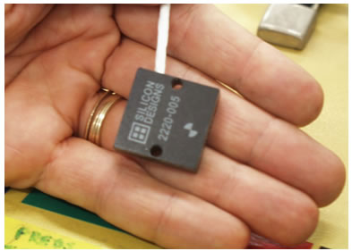
Figure 12. Photo. Silicon Designs model 2220 accelerometer.
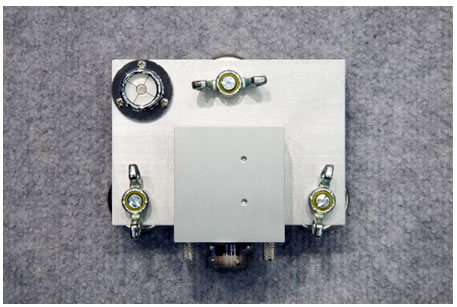
Most accelerometers are not very shock resistant, and dropping them is usually fatal. Due to hydraulic damping, specifications for the Silicon Designs accelerometer indicate that the 5-g unit is resistant to a 2,000-g shock. During the research, an accelerometer box was unintentionally dropped onto a concrete floor from a height of 30 inches (760 mm), and it survived without any measurable effect on its calibration. Figure 13 shows an accelerometer box on a calibration platter.
Figure 13. Photo. Accelerometer box on calibration platter.
The Silicon Designs accelerometer is a microelectromechanical systems (MEMS) device. As a result, it produces a signal due to the acceleration of Earth’s gravity. This is termed the zero bias by the manufacturer. It is advantageous because it allows researchers to use Earth’s gravity to calibrate the accelerometer.
A Vishay 2310 signal conditioner is used to power the accelerometer. The signal conditioner has a six-pole, low-pass Butterworth filter that is set at 1,000 Hz to protect against aliasing by removing unwanted high-frequency electrical noise. The same signal conditioner is also used with the reference load cell, thereby saving on hardware costs.
Calibration of the Accelerometer
The Silicon Designs accelerometer is a nonlinear device. The output is slightly nonlinear with respect to the acceleration. In order to overcome this, the manufacturer defines the following relationship:
Figure 14. Equation. Nonlinear conversion of voltage to acceleration.
Where:
g = Measured acceleration in gravitational units.
V = Accererometer output in volts.
a,b = Coefficients of polynomial from manufacturer’s calibration at 50 Hz.
This relationship is used to convert the accelerometer response (in volts) to engineering units (in gravitational units). The second- and third-order terms contribute a relatively small amount to the conversion.
The accelerometer response is also slightly affected by ambient temperature. This only affects the zero bias, b, and the first order slope, a1. Daily calibration of the accelerometer to a known acceleration (Earth’s gravity) is used to calibrate the output and determine the bias and slope a1 at ambient temperature.
Daily accelerometer calibration is straightforward. The accelerometer is calibrated on a flat and level plate that is also used to store the accelerometer when it is not being used (see figure 13). First, 1s of accelerometer readings (15,000 readings) is taken in a +1 g gravity field. This process is repeated 10 times. Next, the accelerometer (in its protective box) is inverted, and 10 more sets of readings are taken in a -1 g field. The accelerometer is immediately inverted back into the +1 g field, and 10 more sets are read to verify that the hysteresis effect (discussed later) did not cause a significant change in the resulting output.
The standard deviation of each second of data is examined to confirm that the accelerometer was being held steady during the test. Results are also compared to historical data for the accelerometer to ensure that the results are typical. Data from the calibration are used to determine a daily value for the zero bias, b, in gravitational units, and the slope, a1, in gravitational units per volt. These results include the effect of the gain setting in the signal conditioner, temperature effects, hysteresis effects, aging of the accelerometer, and other factors.
Data Checks During Accelerometer Calibration
Several data checks are made during the daily calibration of the accelerometer. Some are performed to ensure that the device is working within normal parameters, and others are used to look for changes from one accelerometer calibration to the next. The data checks are as follows:
Hysteresis of Silicon Designs Accelerometer
The Silicon Designs model 2220 accelerometer encounters problems with hysteresis. Every time the accelerometer is inverted in Earth’s gravity, the zero bias changes. The magnitude of this change increases exponentially with time and occurs whether or not the accelerometer is powered; thus, it is a materials science problem rather than an electrical one. This accelerometer drift could present a biased nonrandom error. If it is not accounted for, hysteresis can lead to a calibration error in excess of 1 percent.
The magnitude of the error changes over time when the accelerometer is at rest in Earth’s gravitation. To overcome this, the accelerometer needs to be kept upright in the +1 g gravity field as much as possible. It should only be flipped upside down during daily calibration. If the time for flip calibration is kept short, the effect on the overall daily calibration is small.
Hysteresis does not affect the dynamic response of the accelerometer during the FWD pulse because it stays in a +1 g overall gravity field. Since Earth’s gravity (a static response) is used to calibrate the dynamic response of the sensor, hysteresis must be accounted for as part of the accelerometer calibration.
Figure 15 and figure 16 show the hysteresis effect measured for one accelerometer. An accelerometer was left in a +1 g condition overnight. Readings were taken for 15 min and were very stable (not shown). Next, the accelerometer was inverted to a -1 g condition, and the voltage output was recorded every second for 30 min. The accelerometer was then returned to a +1 g gravity field, and additional measurements were taken for 15 min (see figure 15).
Each figure shows an immediate change in one direction, with a signal change on the order of 1–1.5 mV. This is followed by a slower long-term change in the opposite direction. If inversion time (during daily flip calibration) is kept under 20 s, the effect on the accelerometer voltage is less than 0.035 percent (about 0.5 mV).
The rate of drift due to hysteresis diminishes with time. After 6 days at room temperature, the accelerometer is completely stable. If the accelerometer is stored upside down for a long period, it takes about 24 h to equilibrate it in the upright position to within 0.1 percent of the stable response. For this reason, the accelerometer should be stored in a +1 g field at all times.
As a general rule, if the accelerometer is inverted for a brief period of time, it should be left in the upright position for an equal length of time to re-equilibrate it. Note that in figure 16, the accelerometer was inverted from the orientation in figure 15, and the time scale was continued.
Figure 15. Graph. Hysteresis effect in a -1 g field.
Figure 16. Graph. Hysteresis effect in a +1 g field.
Temperature and Electromagnetic Interference Sensitivity
The feasibility of using an accelerometer as a reference device for calibrating FWD deflection sensors depends in part on the effects of the environment. If the device is affected too much by temperature or by interference from electromagnetic fields, then the accelerometer could fall short of the ±0.3 percent accuracy required for deflection sensor calibration.
Silicon Designs specifies a scale factor (slope a1) temperature shift between -250 and +150 ppm/°C for model 2220-005 (see figure 17). Two accelerometers (serial numbers 277 and 278) were calibrated over a range of temperatures, and the change in the output voltage was determined. Results show that if the maximum allowable error due to temperature change was 0.1 percent, the maximum acceptable temperature shift was 18 °F (10 °C).
Electromagnetic interference (EMI) has been shown to affect accelerometer measurements when the fields move with respect to the device. Aluminum and steel were tested for use as shielding materials. While a grounded steel box was able to completely defeat the effect of electromagnetic interference (EMI) on the accelerometer, an aluminum box had optimal results in fields above 1 G (0.0001 T) and was deemed sufficient. Even large magnetic fields had a limited effect on the accelerometer readings. A maximum change of 0.04 percent in the voltage output was observed when several high-powered magnets were placed next to the accelerometer. It should be noted that the aluminum box also helps insulate the accelerometer from temperature effects. Temperature measured at the DAQ can be expected to move more rapidly than inside the aluminum box, provided the box is not in direct sunlight.
Figure 17. Graph. Scale factor temperature shift for accelerometer.
Double Integration of Accelerometer Signal
Using an accelerometer as a reference sensor in deflection measurement requires the output to be double integrated from the accelerometer to convert to displacement. This is a challenging problem in part because releasing the FWD mass before the mass strikes the load plate can leave a legacy of ongoing damped vibration in the pavement at the moment the mass strikes.
When considering integration for any purpose, it is necessary to remember that the first integral of a constant is a ramp. That is, ∫A dt = At + B. The second integral of a constant is a parabola, ∫∫A dt = ½ At2 + Bt + C, where A, B, and C are constants, and t is time. In instrumentation engineering terminology, the ramp is the drift, and the parabola is the nonlinear drift.
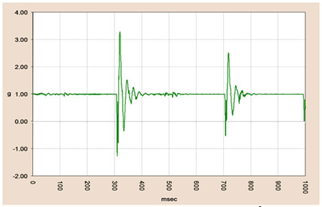
Before performing the integration calculations, several boundary conditions and assumptions must be defined. Figure 18 shows the acceleration trace from a Dynatest® FWD impulse after converting from volts to gravitational units. The release of the mass occurs around 40 ms, and the strike of the mass on the load plate occurs just after 300 ms.
The baseline in figure 18 is on +1.0 g because the MEMS accelerometer responds to Earth’s gravity. This zero bias can be measured by taking a burst of readings before the FWD mass is released. The readings are examined to ensure that no unwanted vibrations are occurring just before the drop. Subsequent acceleration data can be corrected to remove the zero bias before integration (additional details on this process are given in the next section). Figure 19 and figure 20 show the resulting integration of the accelerometer trace, first to velocity and then to displacement.
Figure 21 through figure 23 show a similar set of results for a JILS machine. The peak force for both examples was about 16,000 lbf (70 kN). It is evident that different types of FWDs have different vibration characteristics both before and especially after the falling mass strikes the load plate, which is a challenge to accommodate in the integration routines. A small but acceptable amount of baseline drift can be seen in figure 20 and figure 23.
Figure 18. Graph. Raw accelerometer output from a Dynatest® FWD impulse.
Figure 19. Graph. First integration (velocity) from a Dynatest® FWD impulse.
Figure 20. Graph. Second integration (deflection) from a Dynatest® FWD impulse.
Figure 21. Graph. Raw accelerometer output from a JILS FWD impulse.
Figure 22. Graph. First integration (velocity) from a JILS FWD impulse.
Figure 23. Graph. Second integration (deflection) from a JILS FWD impulse.
The deflection sensor calibration stand experiences a unidirectional acceleration, a(t), in the vertical (z-coordinate) direction. This is measured continuously using the accelerometer that is attached to the stand. The digitized data represent the vector sum of two accelerations: a constant acceleration, ao, due to Earth’s gravity and a variable acceleration, a'(t), due to the impact of the falling mass.
The mass is released at time tr, and the time of impact of the mass is ti, which occurs after the release of the mass. Peak deflection zpeak is at tpeak (marked in figure 20 and figure 23), which occurs after the mass strikes the load plate. Thus, tr < ti < tpeak. The goal is to determine zpeak as accurately as possible.
When the mass goes into free fall, the force of the FWD load plate on the pavement is reduced by the weight of the mass. This causes the pavement to spring up slightly. The KUAB FWD has an outrigger system that supports the mass; hence, there is no change of force at the load plate. The JILS FWD uses a pair of air bags to apply a large preload on the load plate. It also uses a larger mass and a shorter free fall distance than the other types of FWDs, so the damping time between tr and ti is shorter (about 175 ms in figure 23).
If the extraneous vibrations due to the release of the mass are damped out before ti, the combined acceleration after ti is as follows:
Figure 24. Equation. Acceleration due to gravity and the FWD load pulse.
Where:
a(t) = Acceration over time t.
a0 = Constrant acceration due to Earth’s gravity.
a’(t) = Acceleration due to the FWD mass strike at ti
The constant, ao, is measured by averaging a burst of 3,000 readings taken immediately before the mass is released (at that time, a’(t) = 0). If the calibration stand is not exactly vertical or if the temperature has changed since the accelerometer was last calibrated, ao will include these effects. Since ao can be measured precisely and its value is subtracted from all subsequent accelerometer readings taken before and after the mass is released, this leaves a relative acceleration, a’(t) = a(t) – ao. Thus, the equation in figure 24 becomes the following:
Figure 25. Equation. Relative acceleration after removing Earth’s gravity.
The relative acceleration in figure 25 can be integrated to find the velocity as a function of time, v(t) (see figure 26).
Figure 26. Equation. Velocity as a function of time.
By examining the data, the starting point of the integration can be chosen on the interval tr < ti so that t = 0 and a’(0) = 0. If v(0) = 0 (i.e., there is no initial velocity of the pavement at t = 0), then constant c1= 0. Hence, the deflection over time z(t) becomes the following:
Figure 27. Equation. Deflection as a function of time.
Again, t = 0 is chosen so that v(t) = 0, and if z(0) = 0, then c2 = 0. The starting point for integration in figure 26 and figure 27 will most likely not be at the same reading number in the data file. If there is also a time-variable acceleration ao(t) and/or a time-variable velocity vo(t) (e.g., residual vibration in the pavement caused by the decrease in force when the mass is released or due to the FWD vibrating after the release) at the start of integration, then figure 26 becomes the following:
Figure 28. Equation. Velocity with initial vibration.
Where:
v(t) = Velocity over time
v0(t) = Initial time-variable pavement velocity (vibration).
a0(t) = Initial time-variable pavement acceleration (vibration).
The accelerometer measures the combined vector a(t) = ao + ao(t) + a’(t). ao can still be measured at a time when ao(t) + a’(t) = 0. A starting point can also be chosen for the integration such that ao(0) + a’(0) = 0. However, v(0) is not likely to be zero at t = 0, and vo(t) and ao(t) are unknown functions, so it becomes difficult to solve the equation in figure 28. It is even more difficult to define z(t).
If there is vibration present at ti but it is still assumed that figure 26 and figure 27 are applicable, the constants will be nonzero. It is not possible to separate ao(t) and a’(t) in the accelerometer data, and vo(t) is an undefined function. Thus, z(t) will contain nonlinear drift.
The vibration functions vo(t) and ao(t) may be nearly fully damped at the starting point t = 0, in which case, the drift may be small, and the error of the peak deflection zpeak may also be small and possibly of random magnitude. However, if the vibrations are renewed and enhanced when the falling mass strikes the load plate at ti, then vo(t) and ao(t) may be significantly nonzero, and the drift and the error in zpeak may become large. The vibration functions vo(t) and ao(t) may be nearly fully damped at the starting point t = 0, in which case, the drift may be small, and the error of the peak deflection zpeak may also be small and possibly of random magnitude. However, if the vibrations are renewed and enhanced when the falling mass strikes the load plate at ti, then vo(t) and ao(t) may be significantly nonzero, and the drift and the error in zpeak may become large.
The best approach is to only perform the double integration in an environment where the vibration due to the release of the FWD mass is essentially zero. Then, both ao(t) and vo(t) will be zero, or nearly so, and will contain little if any drift. To ensure that condition is met, the accelerometer signal can be analyzed during each drop for a short period before ti and all drops that show excessive vibration can be rejected.
Research for this study has shown that it is important for the FWD to be level and seated squarely on the pavement to minimize undesired vibrations. Several seating drops (no data recorded) should be performed before data collection to establish good contact of the load plate. For the Dynatest® and Carl Bro FWDs, it is necessary to lubricate the load plate swivel, and it must be free to rotate. For the JILS FWD, which does not have a swivel, it is important to verify that the load plate is properly seated while the mass is in free fall. This can be accomplished using a sheet of paper, and the procedure for checking proper seating is explained in more detail in annex 3 of appendix A.
WinFWDCal is used to implement data acquisition and double integration. It also provides several QC checks during data processing. An earlier section discussed setting the trigger level. The following steps are taken when the calibration operator initiates an FWD drop during reference calibration.
Measuring ao
Before the computer screen turns green around the perimeter, which is a signal to the FWD operator to release the mass, the computer takes a burst of 3,000 readings at 15,000 Hz (200-ms read time) and computes the average (ao) and standard deviation. If the standard deviation is larger than 0.005 V, a popup message alerts the user that the predrop vibration exceeds the acceptable level.
The readings are converted to gravitational units, and the vector is checked to ensure that all readings are between 0.98 and 1.02 g. According to NIST, the acceleration of gravity (1 g) equals approximately 32.2 ft/s2(9.80665 m/s2).(16) In Minneapolis, MN, gravity is approximately 32.2 ft/s2 (9.80585 m/s2); in Denver, CO, it is approximately 32.1 ft/s2 (9.79615 m/s2); and in College Station, TX, it is approximately 32.1 ft/s2 (9.79324 m/s2). Gravity is not less than 0.9985 g in any of these locations. If the data are out of range, the accelerometer is not working correctly, and a popup message alerts the calibration operator. Data for the drops are saved in the time history file.
Finding the Trigger Point
Incoming readings from the accelerometer are continuously scanned for the trigger level. When 10 consecutive readings are over the trigger level, the trigger is satisfied. This process avoids a false trigger due to a voltage spike or other anomaly.
After the trigger is satisfied, at least 10,000 more readings are collected and saved in buffers. Accelerometer readings measured in volts are then transferred from buffers to a program array such that the trigger point is the 5,000th reading out of 15,000. Thus, 0.333 s of data are ahead of the trigger, and 0.666 s are after the trigger. The raw data in volts, the absolute acceleration in gravitational units, and the relative acceleration in gravitational units are saved in the time history file for the drop.
Finding the Time of Impact, the Time of Peak, and the Pulse Rise Time
The time of impact, ti, is determined by working backward in time from the trigger point. Researchers seek to find the transition point from where the deflection time history trace is steep to where it is level by examining the standard deviation of sets of 25 readings. In figure 23, ti is located at the first X around 300 ms.
The standard deviation of the previous 25 readings is calculated and placed in an array. Moving back one point, the standard deviation of the next set of 25 readings is calculated. Similarly, the running standard deviation of consecutive sets of 25 points is tabulated.
When the standard deviation falls below 0.020 g, it indicates the time of impact. A secondary check is made to assure that the acceleration at that point is not less than -0.030 g. If it is not satisfied, researchers must continue to work backward until both criteria are satisfied.
The time of peak, tpeak, occurs at the first maximum reading after the trigger point. Pulse rise time can be calculated by subtracting ti from tpeak. Rise time is reported on screen for each drop by WinFWDCal.
Finding the Starting Points for Integration
The starting point for integration of the acceleration data to velocity is determined by working backward from ti. The first set of three consecutive readings where the acceleration is within ±0.0030 g is found. The starting point for acceleration integration is assigned as the middle reading of the three. The reading number is recorded in the time history file.
The starting point for integration of velocity data to deflection is accomplished in a similar manner using the velocity data array. Working back from ti, the first set of three consecutive readings where the velocity is within ±30 μm/s is found. The starting point for velocity integration is assigned as the middle reading of the three. The reading number is recorded in the time history file.
Generally, the two starting points occur at different reading numbers. For both the acceleration and the velocity data arrays, if a starting point cannot be located within 50 ms ahead of ti, a popup error message indicates excessive vibration before the strike of the mass. In this case, the data for the drop should be rejected, and the drop should be repeated.
Performing the Integration
Integration involves computing the area under a curve. Over a period of 1 s, 15,000 readings are taken, so the readings are 0.0667 ms apart. The digital integration is computed by averaging two adjacent readings and multiplying by the time interval. The running sum is computed by adding these areas forward and backward from the starting point. By definition, the sum at the starting point is zero.
The development of a multiple-sensor stand contributed to the project’s goals of expediting the calibration process and creating a universally compatible procedure. The multiple-sensor stand can save time during calibration by eliminating the need to reference calibrate deflection sensors individually. The design of the stand allows it to be positioned close to the load plate for all brands and models of FWDs.
Under the new calibration protocol, the sensors only need be repositioned once during reference and relative calibration by performing a vertical inversion with respect to the location of the accelerometer. This ensures unbiased results from positions on the lower half of the stand to those at the top. In the case of a KUAB seismometer FWD, horizontal rotation of the stand removes the effect of the two columns of the stand.
Photos of the two stand designs are provided in figure 59 and figure 68 of appendix E. Details about installing and using the stands are provided in appendix F.
Column Design
After examining three different geometries of multiple-sensor stands, the vertical column or "ladder" design was found to be the best option. Its welded aluminum construction is lightweight, and it is stiff enough to ensure consistent deflections for all positions in the stand. Additionally, it is the least affected by the rolling motion of deflection waves.
For the new AASHTO R32-09 protocol, it was necessary to develop two different stands, one for geophones and another for the seismometers used by KUAB FWDs.(1) A total of 10 geophones or seismometers can be simultaneously calibrated using the new stands, and the same stand can be used for both reference and relative calibration.
Ball-Joint Anchor
To ensure accurate measurement with the columnar stand design, it is necessary to anchor the stand firmly to the test pad. Early tests on a variety of prototype stand designs involving an uncoupled anchor showed that testers could not provide enough downward force to keep the stand in contact with the test pad and produce consistent results. The graph in figure 29 shows the results of the tests.
Coupling the anchor to the floor is only an issue when performing the single inversion procedure. Monthly calibration with full rotation allows the use of an uncoupled stand since all sensors are in all positions in the stand, and the effects of position in the stand are accounted for.
Two methods of attaching the calibration stand to the floor were investigated. One approach was to bolt the stand directly to the pad with one or two anchors. The other method was to connect the stand through a ball-joint clamp bolted to the pad (see figure 53 in appendix E). The single-hole direct anchor was acceptable in terms of unattributed (or residual) error and range of deflections, as was the ball-joint anchor. The ball-joint anchor was selected over the direct anchor for the following reasons:
Figure 29. Graph. Comparison of sensor stand performance.
The reference load cell has been modified in two ways. The thickness of the lid was increased from 0.625 to 1 inch (16 to 25.4 mm) to better resist bending and permanent deformation. The guide fingers were moved back slightly from an 11.7-inch (300-mm) diameter to an 11.89-inch (305-mm) diameter to accommodate the slightly larger load plate on JILS FWD.
When calibrating the reference load cell, the maximum load was increased from 20,000 lbf (89 kN) used in the SHRP protocol to 24,000 lbf (107 kN). This change was made to accommodate the higher preload pressure used by the JILS FWD. The calibration of the reference load cell should be performed by a qualified agency in accordance with AASHTO R33-03.(10)
A new design for the reference load cell with a significantly higher load capacity for use with HWDs was investigated. The design used an array of three commercially sold load cells with a combined load capacity of 90,000 lbf (400 kN). However, the concept was not successful because each of the three load cells had a slightly different sensitivity in terms of force per volt. When combined with slight variations in the flatness of the test pad and small eccentricities of loading from FWD, the resulting calibration factor was sensitive to the orientation of the reference load cell.
Overcoming this problem would require that each load cell have its own signal conditioner. The DAQ would read each channel, and the computer would sum the three loads. This made the endeavor prohibitively expensive and too complicated, so the project was abandoned.
One task was to update the existing software to a modern Microsoft Windows®-based graphical user interface and eliminate the need for manual data entry. While there will always be ongoing updates to any software as complicated as WinFWDCal, the original goal was met.
The programming language for WinFWDCal is Microsoft Visual Basic 6.0®. It was chosen because it did not require a complete rewrite of the original code, which used Microsoft QuickBasic® language. Also, the KUSB data acquisition card had drivers for Microsoft Visual Basic 6.0®.
The update of the program started in June 2005 with the conversion of the FWDREFCL code to Microsoft Visual Basic 6.0®. By the time this was completed, the accelerometer and data acquisition systems had been chosen, and the proof of concept for the double integration method had been accomplished using LabVIEW in October 2005.
A draft Microsoft Visual Basic® program that performed some of the basic data acquisition functions and analysis was used during visits to the FWD calibration centers in April and May 2006. The objective of the visits was to test the software with all four types of FWDs. Comments by the calibration operators and other people who participated were incorporated into the program.
Results with WinFWDCal were checked using spreadsheets and Minitab® statistical software, as well as by hand to confirm their validity.(16)
The beta version of WinFWDCal was vetted at Cornell University prior to its release to the four regional calibration centers in late November and early December 2006. Periodic updates of WinFWDCal have been issued on a roughly quarterly basis. Version 2.0 of the software was released in December 2009. It incorporates some user-suggested improvements that make the calibration setup easier to navigate. Version 2.0 also provides software support for monthly relative calibration using the manufacturer-provided calibration stands.
Electronic Data Transfer
A problem was encountered with transferring data from an FWD to WinFWDCal. Each type of FWD has a different native file format, and several manufacturers have many different formats. The AASHTO PDDX file standard was chosen as the preferred format for data transfer after discussion with the FWD manufacturers, calibration operators, and other FWD users.(7) This led to the development of a stand-alone program, PDDXconvert. WinFWDCal uses PDDXconvert as an intermediary for all data transfers.
A data file is copied in native format onto a USB flash drive or a floppy disk to transfer data from the FWD to the calibration computer. This eliminates the manual entry of data into the calibration software, which, in turn, saves time and reduces human error as a factor in the calibration procedure. PDDXconvert reads the file and converts it to a common format that WinFWDCal can read and use.
PDDXconvert does not solve all of the problems of electronic data entry to WinFWDCal. More data than just the sensor readings are needed for FWD calibration. Information such as the FWD model identification, FWD operator name, sensor serial numbers, current sensor gain factors, and last calibration date are needed for record keeping and for the certificate of calibration. A revised and more comprehensive standard is needed for the PDDX file format. A recommended new standard, based on experience working with various FWD native file formats and many user needs, is provided in appendix C.
Two FWD calibration data exchange file formats are described in appendix C. One format provides a suggested file name and contents for exchange of information from FWD that is needed by WinFWDCal. The other details the layout of an electronic file that is created by WinFWDCal that can transfer the calibration results to the FWD. The FWD manufacturers need to provide the means to create the first file and to read the second one.
Historical Database of FWD Calibrations
During the development of the new calibration protocol, each of the existing FWD calibration centers in the United States was asked to provide records of all calibrations performed there, and data were combined into a database of historical results. The data were reviewed to see if annual calibration is warranted. The results showed that changes in the sensor gains occur continuously, and annual calibration is needed to ensure that accurate data are collected by FWDs.(4)
The review found that some deflection sensors have gain settings outside the recommended range of 0.98 to 1.02 (which comes from the manufacturer’s specifications). However, many of these sensors are stable from year to year. Since the calibration factors correct the measurement errors, there is no need to replace sensors that are stable.
Stability over time is more important than whether the gain factor falls between 0.98 and 1.02. Evaluation of the historical database showed that an individual gain factor does not change more than 1 percent from one calibration to the next (typically 1 year apart). This result is used as the first criterion in evaluating and accepting the results of an FWD calibration.
When data for a particular FWD are available for 4 years or more, the long-term data can also be used as part of the calibration acceptance criteria. From the historical database, it was found that an individual gain factor should change no more than 0.3 percent per year, provided that at least three calibrations were done in the 4-year period.
The long-term allowance for change (0.1 percent) is less than that for a single year (1 percent) because short-term change is usually more volatile than long-term change. Given that the random variability of two repeat calibrations is 0.3 percent, it makes sense that a long-term series of calibrations would show less variability.
In spite of the existence of the historic database, it will be difficult to implement the long-term acceptance criterion until the new AASHTO procedure has been in use for 4 years or longer for several reasons. Although the new calibration procedure is similar to the old SHRP procedure, there are many differences. Beam movement was a factor in the old procedure, and it has been eliminated in the new procedure. Additionally, there are only a small number of FWDs that have 4 years of calibration history, and essentially all of those machines were Dynatest® FWDs.
The objective of creating the new procedure was to make improvements without sacrificing the quality of the calibration. In order to compare the results of the old and new procedures, two large sets of replicate calibrations were collected—one using the older SHRP protocol and the other using the newly developed AASHTO R32-09 method.(1)
The same FWD was used for all of the calibrations. The data using the old procedure were taken in early 2006, and the new procedure was used in late 2006. The FWD sensor gain factors that were in place before the data collection began were left in place throughout all of the testing.
Influence on Deflection Sensor Gain Factors
Nine calibrations of the nine geophone sensors were completed using each protocol. The overall average gain obtained with the new AASHTO protocol was 0.26 percent higher than the average gain using the older SHRP protocol. The difference was statistically significant. The variance of the calibrations was the same for each protocol.
Figure 30 shows a comparison of the results for the two protocols. The upper half of the graph shows the final gain with the old SHRP protocol, and the lower half shows the results with the new AASHTO protocol.
Figure 30. Graph. Deflection sensor final gain values produced with the old and new protocols.
Influence on Load Cell Gain Factors
In total, 20 load cell calibrations were completed with the old SHRP protocol, and 17 were completed with the new AASHTO procedure. Figure 31 shows the load cell final gains for the old and new protocols. The average final gain increased by 0.4 percent. The 95th percentile confidence interval on the difference in the final gain was 0.27 percent. Thus, the difference was statistically significant. The variance of the calibrations was the same for each protocol.
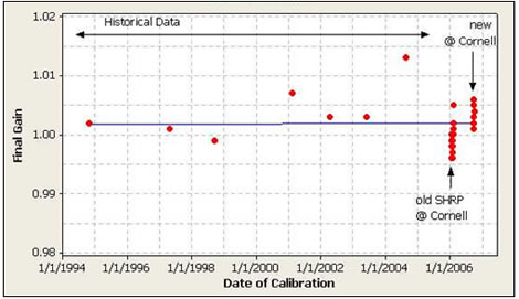
This difference was more than expected. Unlike the hardware and procedural changes that may have affected the deflection sensor gains, there was no significant change in the load cell calibration procedure in the new protocol. The long-term history of the load cell calibrations for the FWD was researched going back to 1994 to see if there was any explanation for the gain change by 0.4 percent.
The gain factor history is shown in figure 32. The year-to-year changes are much more volatile than the long-term trend, which is normal. The calculated trend line is essentially flat. The set of calibrations in early 2006 which used the old SHRP procedure tended to fall mostly below the trend line. The data for the new procedure tended to fall mainly above the trend line.
Figure 31. Graph. Individual value plot of load cell final gain values from the old and new protocols.
Figure 32. Graph. Load cell calibration history from 1994 to 2006.
Therefore, both protocols may have accurately reported the gain factors that were applicable at the time. It is believed that the response of the FWD load cell actually changed during the course of the year. The magnitude of the change found in 2006 was consistent with the changes that have been observed in earlier years. Other interpretations of the data are possible, but from a practical point of view, the results by the new procedure are credible.
Significance of the Differences
The differences in the calibration results using the two protocols were statistically significant. One conclusion from this may be that the new AASHTO protocol yields different results than the old SHRP protocol, but in practical terms, the differences are small. For example, for a deflection of 20 mil (500 μm), the average difference in the two protocols is only 0.05 mil (1.3 μm). It is questionable whether such a small difference has practical meaning, even if the statistics indicate it is significant. Additional differences include the following:
It is possible that the new procedure is more accurate than the old SHRP procedure. The differences are consistent with the expected standard deviation for multiple calibrations. It is also encouraging that the variances were the same by each method. From a practical perspective, the small differences are not a concern.
The pooled fund study focused on removing any possible bias error in the gain factors. Research found that no meaningful bias comes from either the load or deflection calibration procedures. The data cited in the previous section was used to formulate a precision and bias statement according to ASTM E-177.(17)
Using ASTM E-177 terminology, repeatability is defined as the overall variation expected at an individual FWD calibration center for all operators. Reproducibility is defined as the expected variation between single tests performed at multiple FWD calibration centers. Thus, repeatability was studied, but there is no information about reproducibility.
The series of calibration trials using the new procedure were used to define the precision and bias. The Dynatest® FWD was used for these tests. Multiple operators were involved to see if there was any difference between calibration operators. The calibrations were completed as quickly as possible (over a period of approximately 3 weeks) to minimize possible changes in the FWD.
Since this testing was on a single Dynatest® FWD at one location, the results should not be applied directly to all brands of FWDs or to multiple centers. However, the historical information about FWD calibration collected by Orr and Wallace and reviewed as part of this research shows that similar results can be expected for most other Dynatest® FWDs.(4)
In total, 17 load cell calibration trials were completed by 3 FWD calibration operators. No differences between operators were found. The overall standard deviation of the final calibration factor was 0.00152. The 95 percent repeatability using a student’s t-test used a multiplier
Precision and Bias Statement for Dynatest® Load Calibration
The 95 percent repeatability of the final gain factor for Dynatest® load calibration is 0.321 percent. There is no bias expected in the final gain factor. No reproducibility statement.
Nine geophone calibration trials were completed by three calibration operators. No differences between operators were found. The overall pooled standard deviation of the final calibration factors for all nine geophones was 0.00245. By using the pooled standard deviation, the normal distribution multiplier of 1.96 may be used.
Precision and Bias Statement for Dynatest® Geophone Calibration
The 95 percent repeatability of the final gain factor for the Dynatest® geophone calibration is 0.480 percent. There is no bias expected in the final gain factor. No reproducibility statement is available at this time.
A key support function under this pooled fund study is the annual QA and certification reviews at each center. These visits help keep each operator informed about the changes in the protocol, equipment, and software. They also ensure that the calibration procedures are being carried out correctly. The annual visits also promote communication and feedback, helping identify needed improvements in the software and the protocol based on operator experience.
QA procedures were developed in the early 1990s beginning with SHRP to be used annually at the FWD calibration centers. The procedures were reviewed and updated as part of the support function of the pooled fund study. During March and April 2008, the first QA visits were conducted. A report for each separate visit was sent to the calibration center and copied to FHWA. Each calibration operator received a certificate of compliance, which was valid for the following year. The certificate conveys that the person performing the calibration is knowledgeable about the procedure.
Two checklists have been developed for use during the QA reviews. One is for reviewing the facilities and equipment, and the other is for reviewing the operator’s performance. The findings are reviewed with the calibration operator, and they become part of the QA visit report. Details about the QA procedures and examples of the checklists are included in appendix D.