U.S. Department of Transportation
Federal Highway Administration
1200 New Jersey Avenue, SE
Washington, DC 20590
202-366-4000
Federal Highway Administration Research and Technology
Coordinating, Developing, and Delivering Highway Transportation Innovations
| REPORT |
| This report is an archived publication and may contain dated technical, contact, and link information |
|
| Publication Number: FHWA-HRT-10-035 Date: September 2011 |
Publication Number: FHWA-HRT-10-035 Date: September 2011 |
A potential shortcoming of the predictive models that rely on the binder |G*| is the need for the moduli to fall within the complete range of conditions under which the material mixture modulus can be predicted. This range of conditions typically includes temperatures from 14 to 129.2 °F (-10 to 54 °C) and frequencies from 25 to 0.1 Hz. All of the possible combinations of these temperatures and frequencies should be known in order to effectively use the predictive equations for pavement design purposes. The specification data cover the necessary range, but four main problems arise in using the specification results to determine the material properties: (1) the availability of data at only a limited number of temperatures, (2) the evaluation of LVE properties at only a single frequency or time, (3) the mixture of time domain and frequency domain measurements, and (4) a mixture of characteristic behaviors under different aging conditions. It is possible to measure the material properties at a sufficient number of frequencies/times and temperatures to perform the appropriate analysis. However, this process is not part of standard agency practice and, therefore, is not included in the current LTPP database.
In this appendix, a combined phenomenological and mechanical approach is developed and presented. This approach, when coupled with a standard optimization technique, can be used with the existing specification test results to determine |G*| over the necessary range. This approach provides sufficient information for |E*| predictions without increasing the testing requirements. This analytical methodology, although more complicated than that typically used in agency offices, may be coded into a software package or a spreadsheet to allow easy, direct, and rapid characterization.
In asphalt binder testing, two TPs are used to extract the LVE properties of the material. At high and intermediate temperatures, DSR is used, and at low temperatures, BBR is used. To determine the properties of a material over an entire range of in-service conditions, results from these two TPs must be combined. The purpose of this section is to present a method that combines these two outcomes into a single relationship.
A comparison of the mastercurve and the t-T superposition shift factor function development with and without BBR data is also presented. The methodology used for mastercurve and t-T shift factor function development using DSR and BBR data generally follows the method presented by Kim et al.(49) The method used herein differs from the Kim et al. method in that it makes more extensive use of optimization techniques.
Significant literature exists on the development of mastercurves from DSR measurements. Stiffness values at multiple combinations of temperature and frequency, such as those shown in figure 80, are first determined via experimentation. The data are then horizontally shifted by temperature along the logarithmic frequency axis to form a continuous function (see figure 81). The amount of horizontal shift is the t-T shift factor for that particular temperature and the shifted frequency is referred to as the “reduced frequency.” This operation is expressed mathematically in equation 59, and an example function is shown in figure 82.
| (59) |
Where:
| aT | = | Time-temperature shift factor. |
|---|---|---|
| ωT | = | Frequency at the physical temperature. |
| ωTR | = | Reduced frequency of ωT at the reference temperature. |
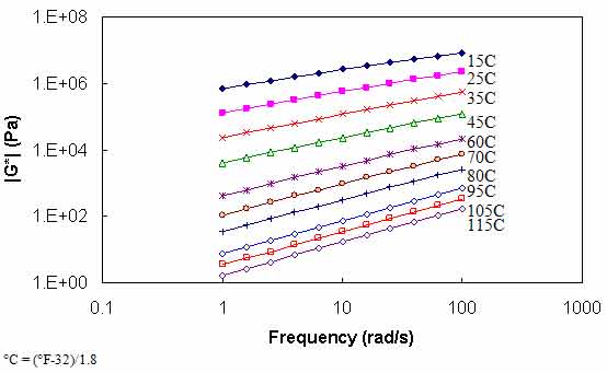
Figure 80. Graph. |G*| versus frequency curves at different temperatures.
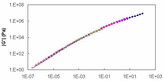
Figure 81. Graph. |G*| versus reduced frequency mastercurve at 59 °F (15 °C).
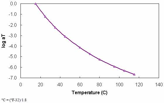
Figure 82. Graph. t-T shift factor function at 59 °F (15 °C).
Prior to desktop computers and optimization spreadsheet functions, the determination of the shift factors and the functional form comprised distinct steps. However, a current common technique is to assume some functional form for the mastercurve a priori and then optimize the coefficients of this function along with either the t-T shift factors directly or a function that relates these factors. Equation 60, which is an extension of the CAM model developed through the SHRP program, is assumed for the mastercurve, and the Williams-Landel-Ferry (WLF) model is assumed for the t-T shift factor function (see equation 61). For all cases, 59 °F (15 °C) is taken as the reference temperature (i.e., aT = 1 at 59 °F (15 °C)).
 |
(60) |
Where:
| Gg | = | Maximum shear modulus or glassy modulus (pascals). |
|---|---|---|
| ωR | = | Reduced frequency (rad/s). |
| ωc, me, and k | = | Fitting coefficients. |
| (61) |
Where:
| aT | = | t-T shift factor at temperature T (°C). |
|---|---|---|
| TR | = | Reference temperature (°C). |
| C1 and C2 | = | Fitting coefficients. |
To utilize the BBR data in |G*| mastercurve development, the data must be further processed because BBR measurements are taken in the time domain whereas DSR measurements are taken in the frequency domain. Also, BBR measurements are taken in the bending mode whereas DSR measurements are taken in the shear mode.
The PG specification defines beam stiffness, S(t), as the inverse of creep compliance, D(t) (see equation 62). The creep compliance values of ALF AC5 at -22, -11.2, and -0.4 °F (-30, -24, and -18 °C) are calculated from the BBR stiffness values and plotted in figure 83. In a manner similar to the mastercurve development method mentioned previously, these curves are horizontally shifted to form a continuous curve. Note that because these measurements are made in the time domain, the reduced time is defined by equation 63.
| (62) |
| (63) |
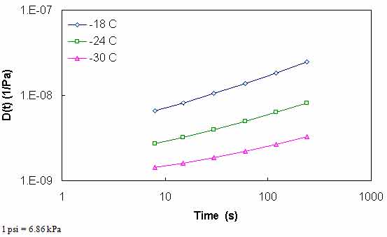
Figure 83. Graph. D(t) at different temperatures for ALF AC5 binder.
For D(t), a generalized power law (GPL) is assumed as seen in equation 64 as follows:
| (64) |
Where D0, D1, and m are regression coefficients. In Kim et al., the determination of the coefficients in equation 64 is shown through a regression technique.(49) For the work presented here, the coefficients are determined via optimization using the Microsoft® Excel Solver function. The two techniques are compared in figure 84 and found to yield indistinguishable results. Note that for the BBR measurements, the t-T shift factors form a linear relationship with temperature as seen in equation 65 as follows:
| (65) |
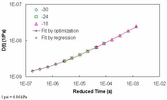
Figure 84. Graph. Comparison of optimization and regression GPL characterization results.
To use the BBR results with DSR measurements, D(t) must be converted to |G*|. To make this conversion, the mathematical consequences of linear viscoelasticity and equation 64 along with equation 66 are utilized. Note that in this process, Poisson's ratio is assumed to be time-independent and has a value of 0.50.
| (66) |
In this equation, n is Poisson's ratio and |D*| is the dynamic axial creep compliance. From linear viscoelasticity, this compliance can be determined by the following relationship:
| (67) |
Where:
| D' | = | First vector component of |D*|. |
|---|---|---|
| D" | = | Second vector component of |D*|. |
Both are defined for the GPL in equations 68 and 69 as follows:
| (68) |
| (69) |
Although it is not necessary for this methodology, the frequencies at which the shear modulus is determined are consistent with LVE time-frequency equivalency principles. The equivalency is given in equation 70 as follows:
| (70) |
To utilize the BBR measurements for CAM model development and t-T shift factor determination, the Microsoft® Excel Solver optimization package is used. In this technique, the coefficients of the CAM model (see equation 60), the GPL model (see equation 64), the WLF equation for t-T shift factors above 32 °F (0 °C), and the t-T shift factor slope for temperatures below 32 °F (0 °C) are simultaneously optimized such that the objective function in equation 71 is minimized. The results from this optimization are shown in figure 85 and figure 86 for the WesTrack binder. Results of the characterization for all binders for a reference temperature of 59 °F (15 °C) are shown in table 37.
 |
(71) |
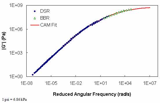
Figure 85. Graph. |G*| mastercurve for the WesTrack binder at 59 °F (15 °C).
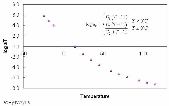
Figure 86. Graph. Optimized t-T shift function for WesTrack binder at 59 °F (15 °C).
| Binder | CAM | t-T | |||||
|---|---|---|---|---|---|---|---|
| Gg (Pa) | fc (rad/s) | k | me | C1 | C2 | C3 | |
| ALF AC5 | 3.60E+10 | 0.06 | 0.0777 | 1.4245 | -13.4747 | 99.8914 | -0.1447 |
| ALF AC10 | 2.49E+10 | 0.09 | 0.0851 | 1.4299 | -12.9868 | 90.7373 | -0.1481 |
| ALF AC20 | 1.81E+09 | 1.60 | 0.1278 | 1.1693 | -13.6667 | 94.2261 | -0.1520 |
| ALF Novophalt | 8.38E+08 | 0.60 | 0.1265 | 1.0477 | -12.6598 | 80.6345 | -0.1624 |
| ALF Styrelf | 8.35E+10 | 0.00 | 0.0622 | 1.2543 | -15.5337 | 121.0536 | -0.1525 |
| MnRd. AC20 | 1.44E+09 | 0.54 | 0.1288 | 1.2208 | -12.6909 | 77.2684 | -0.1638 |
| MnRd. Pen120-150 | 4.04E+10 | 0.11 | 0.0842 | 1.4556 | -12.1122 | 78.8723 | -0.1453 |
| WesTrack | 1.17E+09 | 0.60 | 0.1411 | 1.1828 | -12.9616 | 73.4526 | -0.1547 |
|
1 psi = 6.86 kPa |
|||||||
The methodology presented in the previous section has also been performed using only the DSR measurements. In this analysis, only the CAM model coefficients and WLF model coefficients are allowed to change, and the objective function is modified to that (see equation 72). The purpose of this analysis is to determine the effect of omitting BBR measurements when determining |G*| values outside the DSR measured range. With this goal in mind, it is assumed that the analysis using BBR data represents the most accurate determination of the |G*| mastercurve.
| (72) |
The calibrated CAM model coefficients and the t-T shift factor function coefficients for each of the binders are shown in table 38. A comparison of the values presented in table 37 and table 38 reveals no consistent trend. In some cases, the values from the calibrated model are higher than those from the BBR-calibrated models (higher Gg and k values and lower me), whereas the opposite occurs in other models. In addition, the t-T shift factor function does not extrapolate well to lower temperatures when only DSR values are used in the calibration. An example of this behavior can be seen in figure 87. However, the figure shows that consistent results between the two characterization schemes occur at the DSR temperatures. To examine the effect of the extrapolation error, the GPL model is fitted to the BBR measurements, and the resulting overlap between the two datasets can be observed. When using the DSR-calibrated t-T shift factors, the BBR data are not continuous with the DSR data (see figure 88). This result suggests that the effect of extrapolating the t-T shift factor function is significant and may lead to errors.
| Binder | CAM | t-T | ||||||||
|---|---|---|---|---|---|---|---|---|---|---|
| Gg (Pa) | fc (rad/s) | k | me | C1 | C2 | |||||
| ALF AC5 | 5.24E+09 | 0.66 | 0.0976 | 1.2887 | -13.2075 | 98.3537 | ||||
| ALF AC10 | 3.60E+10 | 0.62 | 0.0872 | 1.3514 | -13.0002 | 92.7463 | ||||
| ALF AC20 | 1.25E+10 | 0.34 | 0.0968 | 1.2981 | -14.0171 | 98.1479 | ||||
| ALF Novophalt | 3.35E+07 | 1.74 | 0.3069 | 0.8552 | -12.3904 | 79.8044 | ||||
| ALF Styrelft | 4.52E+09 | 0.04 | 0.0824 | 1.1214 | -14.8831 | 108.9959 | ||||
| MnRd. AC20 | 3.72E+10 | 0.57 | 0.0924 | 1.3303 | -13.1226 | 86.8517 | ||||
| MnRd. Pen120-150 | 7.42E+10 | 0.90 | 0.0851 | 1.3752 | -12.1104 | 80.9397 | ||||
| WesTrack | 1.43E+08 | 4.33 | 0.2623 | 1.0068 | -13.1142 | 81.7971 | ||||
|
1 psi = 6.86 kPa |
||||||||||
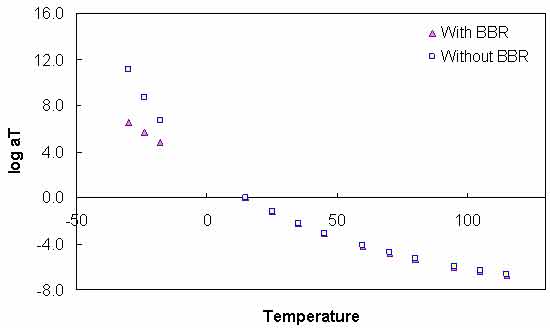
Figure 87. Graph. Comparison of t-T shift factor functions calibrated with and without BBR data.
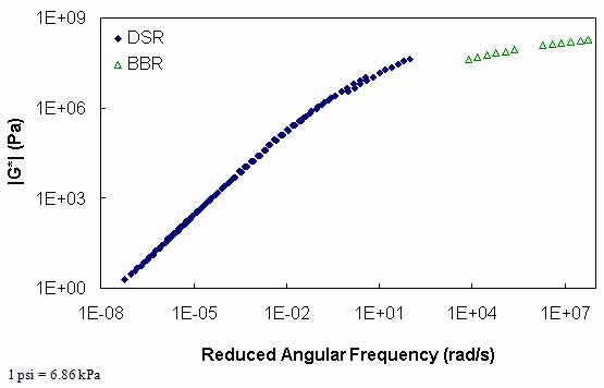
Figure 88. Graph. |G*| mastercurve using t-T shift factor function calibrated without BBR data.
For the purposes of this report, the most critical information is found in the differences between these two techniques at TP-62 temperatures (14, 41, 68, 104, and 129.2 °F (-10, 5, 20, 40, and 54 °C)) and frequencies (25, 10, 5, 1, 0.5, and 0.1 Hz). To explore these conditions, the difference formula shown in equation 73 is utilized for |G*| values that are predicted using the calibrated CAM models at the TP-62 temperatures and frequencies. The results are summarized in table 39 for each of the binders.
 |
(73) |
| Temperature (°C) | Frequency (Hz) | ALF AC5 | ALF AC10 | ALF AC20 | ALF Novochip | ALF Styrene | MnRoad AC20 | Pen 120-150 | Wes Track | |
|---|---|---|---|---|---|---|---|---|---|---|
| -10 | 25 | -11.09 | -153.94 | -211.16 | 87.30 | 29.32 | -629.40 | -334.59 | 67.37 | |
| -10 | 10 | -20.53 | -162.36 | -203.86 | 85.55 | 23.47 | -589.44 | -358.74 | 63.23 | |
| -10 | 5 | -28.23 | -169.15 | -198.98 | 83.95 | 18.73 | -561.10 | -378.72 | 59.42 | |
| -10 | 1 | -48.12 | -186.48 | -189.99 | 78.88 | 6.61 | -501.81 | -431.57 | 47.49 | |
| -10 | 0.5 | -57.59 | -194.67 | -187.24 | 75.91 | 0.90 | -479.17 | -457.47 | 40.55 | |
| -10 | 0.1 | -81.72 | -215.54 | -183.75 | 66.24 | -13.55 | -433.54 | -526.17 | 18.18 | |
| 5 | 25 | 16.83 | -11.35 | -29.59 | 72.25 | 20.04 | -77.81 | -13.86 | 54.92 | |
| 5 | 10 | 14.07 | -9.28 | -22.56 | 67.17 | 15.44 | -58.57 | -10.94 | 50.21 | |
| 5 | 5 | 12.09 | -7.70 | -17.75 | 62.64 | 11.89 | -45.57 | -8.76 | 46.44 | |
| 5 | 1 | 7.96 | -4.02 | -8.19 | 49.60 | 3.57 | -20.03 | -3.78 | 37.54 | |
| 5 | 0.5 | 6.42 | -2.44 | -4.73 | 42.92 | -0.02 | -10.83 | -1.69 | 33.93 | |
| 5 | 0.1 | 3.50 | 1.16 | 1.84 | 25.70 | -8.25 | 7.00 | 2.98 | 27.26 | |
| 20 | 25 | 3.60 | -6.13 | -3.81 | 21.12 | 9.08 | -18.13 | -5.92 | 1.89 | |
| 20 | 10 | 2.11 | -4.30 | -0.90 | 10.85 | 5.61 | -9.73 | -3.60 | -2.43 | |
| 20 | 5 | 1.20 | -2.94 | 0.90 | 3.71 | 3.09 | -4.23 | -1.91 | -4.39 | |
| 20 | 1 | -0.15 | 0.06 | 3.86 | -8.63 | -2.32 | 6.09 | 1.75 | -4.19 | |
| 20 | 0.5 | -0.40 | 1.28 | 4.63 | -11.52 | -4.42 | 9.61 | 3.21 | -2.22 | |
| 20 | 0.1 | -0.24 | 3.92 | 5.42 | -12.25 | -8.72 | 15.95 | 6.27 | 5.47 | |
| 40 | 25 | -3.12 | -2.17 | 3.73 | -17.56 | 3.18 | -1.44 | -1.13 | -20.55 | |
| 40 | 10 | -2.98 | -0.87 | 3.76 | -15.91 | 1.48 | 1.13 | 0.35 | -15.26 | |
| 40 | 5 | -2.66 | 0.05 | 3.52 | -13.42 | 0.38 | 2.60 | 1.37 | -10.88 | |
| 40 | 1 | -1.30 | 1.90 | 2.23 | -5.35 | -1.53 | 4.65 | 3.36 | -0.80 | |
| 40 | 0.5 | -0.49 | 2.56 | 1.41 | -1.57 | -2.06 | 5.01 | 4.04 | 3.10 | |
| 40 | 0.1 | 1.78 | 3.78 | -0.92 | 6.39 | -2.69 | 4.89 | 5.22 | 10.41 | |
| 54 | 25 | -4.30 | -0.72 | 3.71 | -12.03 | 1.64 | 0.44 | 0.31 | -11.80 | |
| 54 | 10 | -3.44 | 0.20 | 2.81 | -7.08 | 0.87 | 1.07 | 1.28 | -6.28 | |
| 54 | 5 | -2.64 | 0.81 | 1.97 | -3.32 | 0.49 | 1.21 | 1.90 | -2.54 | |
| 54 | 1 | -0.39 | 1.87 | -0.37 | 4.40 | 0.19 | 0.58 | 2.90 | 4.19 | |
| 54 | 0.5 | 0.70 | 2.18 | -1.46 | 7.01 | 0.31 | -0.02 | 3.14 | 6.13 | |
| 54 | 0.1 | 3.38 | 2.48 | -4.01 | 10.96 | 1.07 | -1.99 | 3.22 | 8.28 | |
|
°C = (°F-32)/1.8 |
||||||||||
The results in table 39 show that extreme errors may result when using only DSR measurements in the |G*| mastercurve characterization. However, these errors are contained entirely within the low temperature range. At temperatures included in the DSR testing (greater than 59 °F (15 °C)), the errors are small. To place perspective on the differences shown in table 39, the mastercurves for the ALF AC5 and MnRoad Pen 120-150 binders are shown in figure 89 and figure 90, respectively. Note that the mastercurves themselves are calibrated well and that the observed errors are almost entirely related to the t-T shift factor errors (see figure 87). It is interesting to note that the two mastercurves that seem to have the poorest match (i.e., the WesTrack binder in figure 91) do not have the highest error. This result is due to the nature of the error definition and also due to differences in the t-T shift factors obtained from the two characterization methods. This latter effect is seen in figure 89 through figure 91 where all the mastercurves change from an equivalent reduced frequency of 14 °F (-10 °C) and 25 Hz to 129.2 °F (54 °C) and 0.1 Hz. This effect is seen also in the t-T shift factor functions in figure 92 through figure 94.
Furthermore, equation 73 indicates that the error is defined in normal space, and figure 91 indicates that the magnitude of |G*| is smaller for the Westrack binder than for the other binders. If the error is defined in logarithmic space, as seen in equation 74, the error is found to follow the graphical results more closely, as shown in table 40.
The results in figure 89 through figure 94, table 39, and table 40 affect the LTPP database population effort because BBR data are not currently available for any of the LTPP sections. In fact, the only data available in the LTPP database are DSR results at 10 rad/s and limited temperatures. A technique for considering these limited data is presented in the next section. However, these figures and tables reveal that without the BBR test results, the strength of the |E*| predictive models, which rely on the |G*|, would be severely limited at low temperatures.
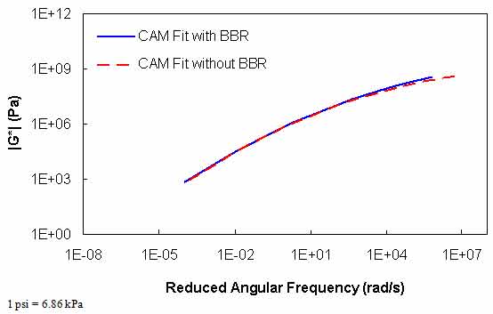
Figure 89. Graph. |G*| mastercurves characterized with and without BBR data for ALF AC5 binder.
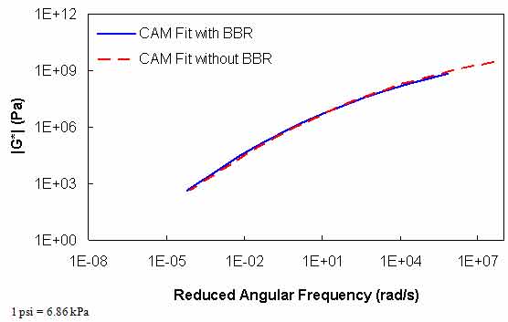
Figure 90. Graph. |G*| mastercurves characterized with and without BBR data for the MnRoad Pen 120-150 binder.
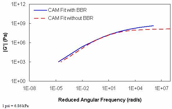
Figure 91. Graph. |G*| mastercurves characterized with and without BBR data for the WesTrack binder.
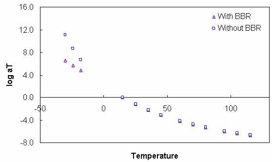
Figure 92. Graph. t-T shift factor function characterized with and without BBR data for the ALF AC5 binder.
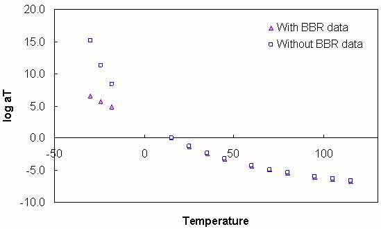
Figure 93. Graph. t-T shift factor function characterized with and without BBR data for the MnRoad Pen 120-150 binder.
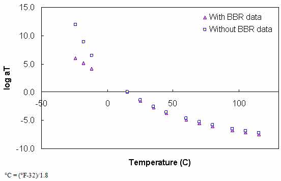
Figure 94. Graph. t-T shift factor function characterized with and without BBR data for the WesTrack binder.
 |
(74) |
| Temperature (°C) | Frequency (Hz) | ALF AC5 | ALF AC10 | ALF AC20 | ALF Novochip | ALF Styrine | MnRoad AC20 | PEN 120-150 | Wes Track |
|---|---|---|---|---|---|---|---|---|---|
| -10 | 25 | -0.54 | -4.06 | -5.16 | 10.71 | 1.75 | -8.35 | -4.65 | 5.97 |
| -10 | 10 | -0.97 | -4.24 | -5.04 | 10.14 | 1.37 | -8.01 | -4.81 | 5.49 |
| -10 | 5 | -1.30 | -4.39 | -4.96 | 9.67 | 1.07 | -7.75 | -4.95 | 5.09 |
| -10 | 1 | -2.12 | -4.76 | -4.80 | 8.43 | 0.36 | -7.14 | -5.31 | 4.09 |
| -10 | 0.5 | -2.49 | -4.94 | -4.76 | 7.83 | 0.05 | -6.89 | -5.48 | 3.62 |
| -10 | 0.1 | -3.39 | -5.40 | -4.71 | 6.29 | -0.70 | -6.32 | -5.92 | 2.44 |
| 5 | 25 | 1.03 | -0.58 | -1.39 | 6.96 | 1.24 | -3.06 | -0.69 | 4.17 |
| 5 | 10 | 0.86 | -0.49 | -1.11 | 6.12 | 0.95 | -2.49 | -0.56 | 3.69 |
| 5 | 5 | 0.75 | -0.42 | -0.90 | 5.47 | 0.73 | -2.05 | -0.46 | 3.34 |
| 5 | 1 | 0.50 | -0.23 | -0.45 | 3.91 | 0.22 | -1.03 | -0.21 | 2.58 |
| 5 | 0.5 | 0.41 | -0.14 | -0.27 | 3.24 | 0.00 | -0.59 | -0.10 | 2.30 |
| 5 | 0.1 | 0.23 | 0.07 | 0.11 | 1.78 | -0.50 | 0.43 | 0.19 | 1.83 |
| 20 | 25 | 0.24 | -0.37 | -0.23 | 1.43 | 0.59 | -1.00 | -0.36 | 0.11 |
| 20 | 10 | 0.14 | -0.27 | -0.06 | 0.71 | 0.37 | -0.57 | -0.23 | -0.15 |
| 20 | 5 | 0.08 | -0.19 | 0.06 | 0.24 | 0.20 | -0.26 | -0.13 | -0.27 |
| 20 | 1 | -0.01 | 0.00 | 0.26 | -0.55 | -0.16 | 0.42 | 0.13 | -0.27 |
| 20 | 0.5 | -0.03 | 0.09 | 0.33 | -0.74 | -0.30 | 0.70 | 0.24 | -0.15 |
| 20 | 0.1 | -0.02 | 0.32 | 0.42 | -0.83 | -0.63 | 1.29 | 0.52 | 0.40 |
| 40 | 25 | -0.24 | -0.17 | 0.28 | -1.15 | 0.23 | -0.11 | -0.09 | -1.35 |
| 40 | 10 | -0.24 | -0.07 | 0.29 | -1.09 | 0.11 | 0.09 | 0.03 | -1.08 |
| 40 | 5 | -0.23 | 0.00 | 0.28 | -0.96 | 0.03 | 0.21 | 0.12 | -0.82 |
| 40 | 1 | -0.12 | 0.18 | 0.20 | -0.43 | -0.13 | 0.42 | 0.33 | -0.07 |
| 40 | 0.5 | -0.05 | 0.26 | 0.13 | -0.13 | -0.18 | 0.48 | 0.42 | 0.29 |
| 40 | 0.1 | 0.21 | 0.44 | -0.10 | 0.63 | -0.25 | 0.54 | 0.64 | 1.16 |
| 54 | 25 | -0.38 | -0.06 | 0.32 | -0.91 | 0.13 | 0.04 | 0.03 | -0.95 |
| 54 | 10 | -0.33 | 0.02 | 0.26 | -0.58 | 0.07 | 0.10 | 0.13 | -0.55 |
| 54 | 5 | -0.27 | 0.08 | 0.19 | -0.29 | 0.04 | 0.12 | 0.20 | -0.24 |
| 54 | 1 | -0.05 | 0.22 | -0.04 | 0.44 | 0.02 | 0.07 | 0.36 | 0.47 |
| 54 | 0.5 | 0.09 | 0.28 | -0.17 | 0.75 | 0.03 | 0.00 | 0.42 | 0.75 |
| 54 | 0.1 | 0.53 | 0.39 | -0.54 | 1.37 | 0.12 | -0.29 | 0.53 | 1.25 |
|
°C = (°F-32)/1.8 |
|||||||||
To fully utilize |G*| in mixture |E*| predictive models, a complete dataset is needed. This dataset must be complete because it must cover the temperature and frequency ranges over which the mixture modulus should be predicted. The full suite of Superpave™ binder specification tests covers this range; however, the data are inconsistent (i.e., |G*| from DSR, and S(t) and m from BBR) and require further processing for complete utilization. This section of the report presents a method for analyzing standard PG binder characterization tests so that the results can provide a more complete dataset.
This method is currently under development by the research team and will be refined as a more complete picture of the available data is obtained. It is assumed that DSR (i.e., |G*|) measurements taken at the standard frequency of 10 rad/s, or 1.67 Hz, at multiple temperatures are available. Results from Superpave TM BBR testing are not necessary in this methodology, but a theoretically justified technique for including such data in the process is shown and evaluated. Currently, such data are not available from the LTPP database; however, the methodology is evaluated nonetheless in case such characterization is included in future research efforts.
To extract a more complete dataset, an analytical expression for |G*| as a function of frequency and temperature must be found. Because asphalt binder is thermorheologically simple, these two factors can be combined into a single parameter, known as “reduced frequency” and shown in equations 75 and 76. Note that although the nomenclature in this report represents frequency using ω, which implies the unit is radians per second, the methodology is equally applicable to frequency in hertz.
| (75) |
| (76) |
Where:
| ωR | = | Reduced frequency. |
|---|---|---|
| aT | = | t-T shift factor, which is a function of temperature. |
This factor can be determined experimentally using results from a temperature and frequency sweep test, such as the test found in AASHTO TP-62.(8) From these tests, the t-T shift factor is determined by horizontally shifting the data at different temperatures until a smooth varying function results. This process is shown previously in this report and is only possible when measurements are taken at multiple frequencies and temperatures.
Measurements from a single-frequency temperature sweep test, such as Superpave™ DSR testing, cannot be used directly to extract these t-T shift factors by simple horizontal translations. This complication arises because the slope of the modulus-temperature relationship, a value that can be determined from single-frequency temperature sweep tests, is dependent on both the frequency and the temperature. Mathematically, this discrepancy can be expressed as follows:
| (77) |
Where:
| T | = | Temperature. |
|---|---|---|
| ωR | = | Reduced frequency. |
| ∂|G*|/∂T | = | Derivative of |G*| with respect to time, known from Superpave™ DSR testing. |
Direct determination is not possible using these measurements, but equation 77 can be solved analytically if functional forms for the t-T shift factor function and for |G*| as a function of reduced frequency are known. In this methodology, the CAM model is assumed sufficient for the latter, and a secondary surrogate model along with the WLF equation is assumed for the logarithm of the former (note that two surrogate models are discussed in the following section). These functions are shown in equations 78 and 79, respectively.
 |
(78) |
| (79) |
Where Gg, ωc, k, C1, C2, and C3 are fitting coefficients. Combining equations 76 and 79 yields the following analytical expression for reduced frequency:
| (80) |
From equation 77, DSR measurements can be used directly to determine the left-hand side of the equation, and the right-hand side can be solved analytically. However, initial trials using this approach proved unsuccessful due to the large spacing between typical Superpave™ DSR measurements. Instead, a more direct approach that uses equation 78 was successful; however, it is necessary to first discuss the model used to predict the t-T shift factors.
Because no clear theoretical link was found between typical DSR measurements and the t-T shift factors, a phenomenological approach and a simple averaging approach were taken. As shown in the following sections, both approaches provide approximately the same accuracy; however, the final recommended procedure will be the subject of further investigation. Because it is important that this t-T shift factor function covers the range over which the mixture modulus would be predicted, only binders with BBR test data have been used. A list of these binders can be found in table 4. For each of these binders, the t-T shift factors were found from optimization fitting using the CAM and WLF equations.
A similarity exists between the normalized shear modulus at 10 rad/s and the log shift factor function. Additionally, a similar relationship exists in the BBR test results at 60 s. These relationships are shown in figure 95 for the binders with BBR test data. For simplicity, both relationships are normalized to |G*| at 10 rad/s at the chosen reference temperature. Because this value is taken as the reference condition and because BBR data are essentially DSR results at 0.01 rad/s (ω=2/π/t), an apparent discontinuity is found in the BBR curve at the reference condition. To understand this discontinuity, it must be recognized that to obtain a given ratio larger than one from DSR test results, the test must be performed at a higher temperature than for a BBR test. This temperature effect is integral to the relationship shown in figure 95 for the DSR results. Because all of the BBR test results are obtained at the same time at 60 s, each is affected similarly, resulting in the discontinuity. However, the slope of this relationship stays much the same as seen in figure 96, where the offset discontinuity in the BBR data has been artificially removed.
It should be noted that the relationships shown in figure 95 have been developed at a reference temperature of 59 °F (15 °C). If DSR measurements are taken at this temperature, then the relationship may be used directly. Alternatively, |G*| at 59 °F (15 °C) may be interpolated if DSR measurements are taken near this temperature. Also, the relationship can be used even if the reference condition is not 59 °F (15 °C), although some error would be inevitable. However, the approach taken here recognizes that at around 59 °F (15 °C) (between 41 and 77 °F (5 and 25 °C)), the t-T shift factors are not significantly different. This relationship follows a second order polynomial, and its implications are shown in the calibrated t-T shift factor relationship shown in equations 81 and 82. The verification of these relationships is shown in figure 97 for FHWA mobile trailer and FHWA ALF binders, which were not included in the calibration process.
| (81) |
| (82) |
Where:
 |
(83) |
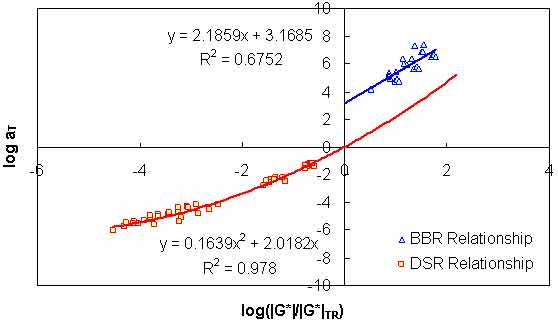
Figure 95. Graph. Phenomenological t-T shift factor function.
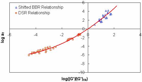
Figure 96. Graph. Effect of change in time from DSR to BBR on the t-T shift factor function model.
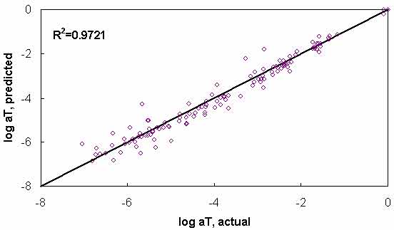
Figure 97. Graph. t-T shift factor model verification with phenomenological model.
A second, more simplistic approach has also shown promise. From the available binder databases, it was found that the t-T shift factor functions are somewhat similar across binder types. In this approach, the same binders used to develop the phenomenological model are processed to find an average representative shift factor function (see figure 98). The advantage of this approach is its simplicity as well as the fact that BBR test results are not needed to obtain a reasonable estimate of the t-T shift factor at low temperatures. Verification of this model is shown in figure 99. Comparing figure 99 to figure 97, it is observed that the average technique has a slightly improved R2 value. In addition, the average technique does not tend to show systematic underestimation of the phenomenological approach in the intermediate temperature ranges. However, in general, the effectiveness of the model does not appear to be significantly superior or inferior to the phenomenological approach. Both are evaluated in the subsequent sections.
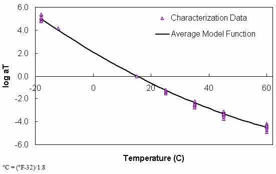
Figure 98. Graph. Average t-T shift factor function.
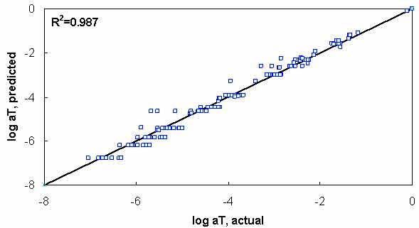
Figure 99. Graph. t-T shift factor model verification with average function model.
Including Superpave™-level BBR data in the optimization process is not as straightforward as the process that combines full DSR and BBR characterization. Complications arise due to the limited dataset that is available (typically only the beam stiffness term, S(t), and m at 60 s for up to three temperatures). Therefore, to use the data as accurately as possible, a few approximate conversion and typical values need to be assumed. The process begins by observing from the theory of linear viscoelasticity that S is actually the inverse of the uniaxial extensional D(t). In order to convert to |G*|, the uniaxial relaxation modulus, E(t), must be found. Because it is possible that only a single BBR test result is available, the conversion technique must be capable of single-point conversion. For this purpose, the approximate relationship given in equation 84 is utilized as follows:
| (84) |
Where n is equivalent to the m-value determined from the BBR test. After determining E(t), the approximate interrelationship in equation 85 is used to convert from time-domain to frequency-domain functions as follows:
| (85) |
Where E'(ω) is the storage modulus. E'(ω) is then converted to the dynamic uniaxial modulus by using equation 86 as follows:
 |
(86) |
Where ø is the phase angle in the material. Experience has found that this value is approximately 24 degrees under BBR test conditions. Therefore, the actual relationship used in this methodology is given by equation 87 as follows:
| (87) |
Finally, to determine |G*|, the mechanistic relationship between uniaxial and shear deformation shown in equation 88 is used. For this relationship, Poisson's ratio is assumed to be time-independent and to have a value of 0.5.
 |
(88) |
Combining equations 84 through 87, the relationship between |G*| and S(t) is given by equation 89, as follows:
 |
(89) |
In addition to calculating the shear stiffness values from beam stiffness and m-values, it is worthwhile to consider fitting the m-values. Recognizing that m-values are the derivative of the logarithm of stiffness with respect to the logarithm of time and that simple multiplicative relationships are used to convert from frequency to time, the analytical expression for the m-value using the CAM model can be given by equation 90, as follows:
 |
(90) |
To develop a complete mastercurve from limited Superpave™ data, the conversion between PAV– and RTFO–aging conditions is necessary. This conversion is also needed in the LTPP database where |G*| values are given in terms of RTFO– and PAV–aging conditions. It is noted that original |G*| values are also available in the database. A similar approach could be used to convert from original (or field–aged) to RTFO. Currently, the more important conversion is from PAV to RTFO. To develop this relationship, the Witczak database binders listed in section 3.0 are used. In general, the relationship between |G*|PAV– and |G*|RTFO is found to be dependent on temperature, frequency, and the chemical properties of the asphalt binder. Because none of the Superpave™ tests directly measure the chemical properties of the asphalt binder, the two primary factors in the PAR model are temperature and frequency. Although not a major factor, the Superpave™ high temperature grade is found to be a secondary factor and may indirectly capture some of the chemical composition effects.
The general form of the PAR model is shown in equation 91 where kT and kω are the temperature and frequency factors, respectively.
| (91) |
In general, kT follows a second order polynomial relationship, with the minimum occurring near the high temperature PG (see figure 100). After calibrating kT, kωis characterized. This relationship follows a power law relationship, with the parameters depending on the high temperature grade of the asphalt binder, as seen in figure 101. With these relationships in mind, equation 91 can be rewritten as equation 92 as follows:
| (92) |
Where T is temperature. Each of the parameters in equation 92 follow a first or second order polynomial according to the high temperature PG of the binder. These parameters are summarized in table 41. The calibration dataset along with the calibrated model are shown according to high temperature PG in arithmetic and logarithmic spaces in figure 102 through figure 105. For model verification, a database of binders obtained from the FHWA mobile trailer and the binders used in the current FHWA ALF study are summarized in table 42. The verification is shown in figure 106 and figure 107, and agreement is found between the model and actual data at all high temperature PG levels.
| PG | β1 | β2 | β3 | γ | τ | λ1 | λ2 | Number of Observations | R2 |
|---|---|---|---|---|---|---|---|---|---|
| 46 | 4.82E-05 | -0.002 | 0.169 | 0.858 | 0.082 | -0.039 | 0.062 | Extrapolated | |
| 52 | 6.08E-05 | -0.006 | 0.359 | 0.842 | 0.082 | -0.043 | 0.180 | ||
| 58 | 7.35E-05 | -0.010 | 0.514 | 0.819 | 0.084 | -0.047 | 0.281 | 429 | 0.983 |
| 64 | 8.61E-05 | -0.012 | 0.633 | 0.790 | 0.086 | -0.050 | 0.363 | 1712 | 0.986 |
| 70 | 9.88E-05 | -0.014 | 0.716 | 0.754 | 0.090 | -0.053 | 0.428 | 182 | 0.937 |
| 76 | 1.11E-04 | -0.015 | 0.763 | 0.712 | 0.095 | -0.056 | 0.474 | 537 | 0.964 |
| 82 | 1.24E-04 | -0.015 | 0.774 | 0.663 | 0.101 | -0.058 | 0.503 | 326 | 0.935 |
| Unknown | 8.21E-05 | -0.011 | 0.641 | 0.787 | 0.082 | -0.033 | 0.689 | 2013 | 0.945 |
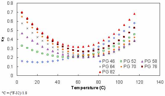
Figure 100. Graph. Effect of temperature on aging ratio of asphalt binder.
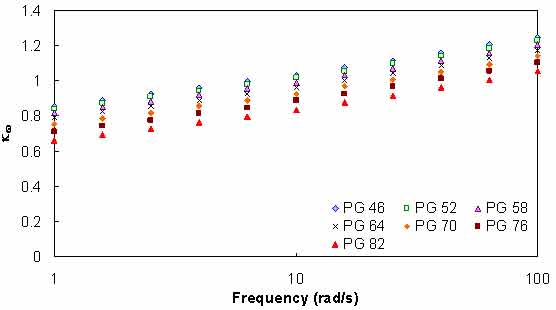
Figure 101. Graph. Effect of angular frequency on aging ratio of asphalt binder.
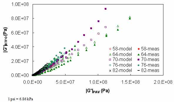
Figure 102. Graph. Calibrated PAR model in arithmetic scale.
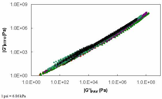
Figure 103. Graph. Calibrated PAR model in logarithmic scale.
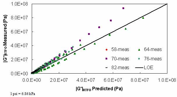
Figure 104. Graph. Strength of PAR model in arithmetic scale.
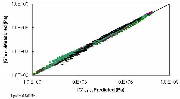
Figure 105. Graph. Strength of PAR model in logarithmic scale.
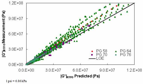
Figure 106. Graph. PAR model verification in arithmetic logarithmic scale.
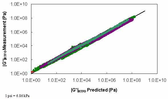
Figure 107. Graph. PAR model verification in logarithmic scale.
| PG | Number of Observations | R2 |
|---|---|---|
| 52 | 297 | 0.702 |
| 58 | 605 | 0.981 |
| 64 | 2289 | 0.970 |
| 70 | 769 | 0.988 |
| 76 | 700 | 0.985 |
Because the DSR data extend only to 59 °F (15 °C), a second relationship must be calibrated for KT at temperatures consistent with the BBR test results. Such a relationship is calibrated by assuming Kω is accurate for BBR conditions and then backcalculating KT from equation 91 and BBR test results under PAV and RTFO conditions. The results suggest that KT changes linearly with temperature under the BBR test conditions and that aging softens the material at the extremely high reduced-frequency region, as seen in figure 108. This observation is confirmed from |G*| mastercurve analysis of the aforementioned binders and is believed to be the first of such an observation. An example of this analysis is shown for the ALF AC 10 binder in figure 109. Due to the limited database, this observation cannot be confirmed with certainty; rather, KT is treated as a fitting parameter, which, along with Kω, approximates the effect of RTFO aging to PAV aging. The complete relationship between RTFO and PAV conditions for BBR tests is given in equation 93, and the parameters are summarized along with the other parameters in table 41. Finally, the calibrated BBR data model is shown in figure 110 and figure 111.
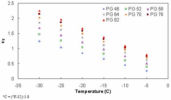
Figure 108. Graph. BBR-calibrated kT relationship.
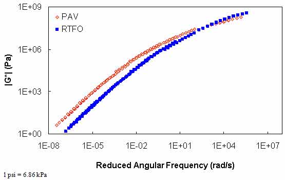
Figure 109. Graph. Comparison of |G*| mastercurve analysis under PAV and RTFO conditions for ALF AC10 binder.
| (93) |
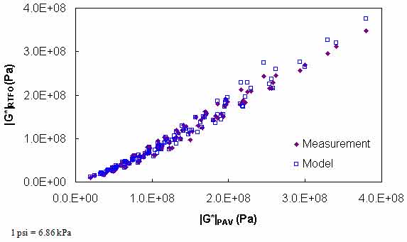
Figure 110. Graph. Calibrated PAR model for BBR conditions in arithmetic scale.
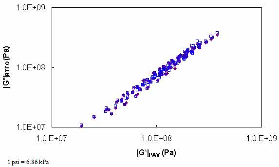
Figure 111. Graph. Calibrated PAR model for BBR conditions in logarithmic scale.
To address the issue of aging effects on the m-value, the PAR model is used to derive the proper relationship. Consider that m, n, the log-log slope of S(t), and |G*|(ω) are close in absolute value at time-frequency equivalency points. In this case, the following equation is considered:
 |
(94) |
Which leads to the following equation:
| (95) |
Casting equation 95 for mRTFO as follows:
 |
(96) |
Applying equation 91 to equation 96 as follows:
 |
(97) |
Simplification leads to the following:
| (98) |
The second term in equation 98 can be solved analytically given the mathematical relationship for provided in equation 92. Performing the differentiation leads to the following:
| (99) |
Equation 99 is verified using the m-values for the binder data in the Witczak database, as shown in figure 112.
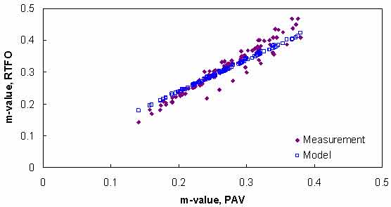
Figure 112. Graph. Verification of m-value relationship.
Verification of the mastercurve construction using only isochronal measurements is divided into three steps. The first verification level (divided into levels 1a and 1b) uses the Witczak binder data, which are also used in the shift factor function model development (i.e., the binder data in table 4 using available BBR measurements). However, this level is not considered true verification because the data were used in the calibration process. Instead, this level assesses the impact of model fitting errors. Levels 1a and 1b differ only in the use of the PAR model. Also, level 1 verification includes BBR data in the analysis process, which is not representative of the currently available LTPP database. However, the second two verification levels are representative of data in the current LTPP database. For sections that have the complete Superpave™ DSR suite, level 2 is the most representative. Sections without the complete high temperature characterization data are better represented by the level 3 verification. Note that for all sections, the phenomenological and average shift factor function models are used and presented.
The first check of these shifting principles consists of a circular check whereby the binders used in the previous section help determine the WLF and CAM model coefficients using only data that would typically be available for Superpave™ testing. For level 1a verification purposes, only RTFO data are used in the analysis; level 1b verification adds an aging model to account for the fact that Superpave™ testing consists of results under original-, RTFO-, and PAV-aged conditions. The steps taken in level 1a verification are as follows:
Typical analysis results are shown in figure 113 and figure 114. In general, the Superpave™ only data analysis results show good agreement with the full analysis results across all of the selected binders. The complete results of level 1a verification are summarized in figure 115 through figure 118 in both normal and logarithmic scales. Overall, the calibrated model fits the data well, with an overall average error of approximately 3.5 percent and a higher average absolute error at 14 percent. These error percentages are comparable for both of the t-T shift factor function models. The major difference between these two models appears to be the tendency of the average shift factor function model to underpredict the modulus values in the high region. Conversely, the average shift factor function tends to show a smaller spread in the prediction error.
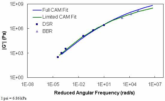
Figure 113. Graph. Comparison of typical |G*| mastercurves characterized using full database and Superpave™ only database.
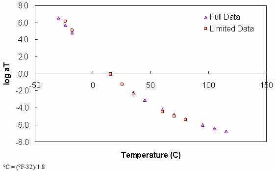
Figure 114. Graph. Comparison of typical t-T shift factors characterized using full database and Superpave™ only database.
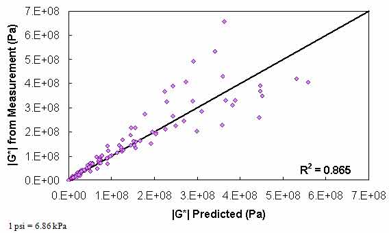
Figure 115. Graph. Level 1a verification of limited data analysis procedure in arithmetic scale using phenomenological shift factor function model.
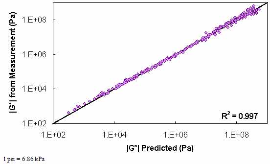
Figure 116. Graph. Level 1a verification of limited data analysis procedure in logarithmic scale using phenomenological shift factor function model.
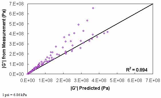
Figure 117. Graph. Level 1a verification of limited data analysis procedure in arithmetic scale using average shift factor function model.
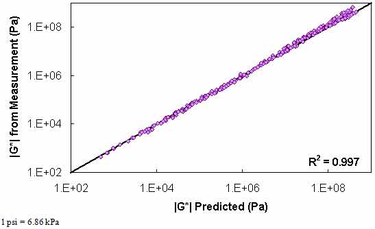
Figure 118. Graph. Level 1a verification of limited data analysis procedure in logarithmic scale using average shift factor function model.
After verifying the limited data shifting procedure, attention is focused on Superpave™ testing on original-, RTFO-, and PAV-aged binders. Because the shear modulus data are desired under the RTFO conditions for the mixture |E*| predictions and because most tests performed on the original-aged binder are also performed on the RTFO-aged binder, the primary model of interest is the relationship between the PAV and RTFO binders. Such a model would then be applied to the DSR tests at the intermediate temperatures and the BBR test results. The steps taken in level 1b verification are as follows:
Typical analysis results for this method are shown in figure 119 and figure 120. A slight decrease in the model strength is observed when compared to the level 1a verification, but in general, the Superpave™ only data analysis results show good agreement with the full analysis results across all of the selected binders. The complete results of level 1b verification are summarized in figure 121 and figure 122 for the phenomenological shift factor function model and in figure 123 and figure 124 for the average shift factor function in both normal and logarithmic scales. Overall, the calibrated model shows an approximately 13 percent error, with the average absolute error higher at 19 percent. As with level 1a verification, these numbers are comparable for both of the t-T shift factor function models. Also, these results tend to show a smaller variability with the average shift factor function model.
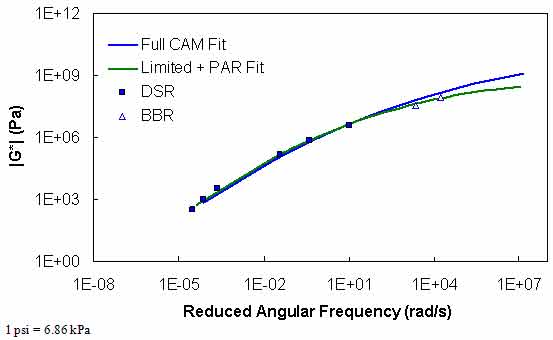
Figure 119. Graph. Comparison of typical |G*| mastercurve characterized using full database and Superpave™ only database plus PAR model.
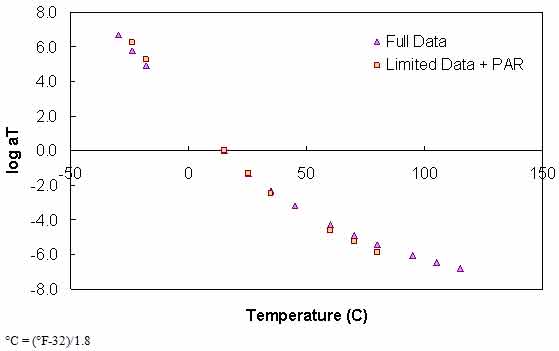
Figure 120. Graph. Comparison of typical t-T shift factors characterized using full database and Superpave™ only database plus PAR model.
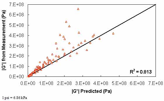
Figure 121. Graph. Level 1b verification of limited data analysis procedure in arithmetic scale using phenomenological shift factor function model.
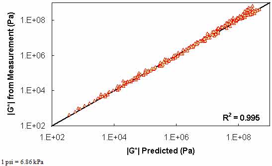
Figure 122. Graph. Level 1b verification of limited data analysis procedure in logarithmic scale using phenomenological shift factor function model.
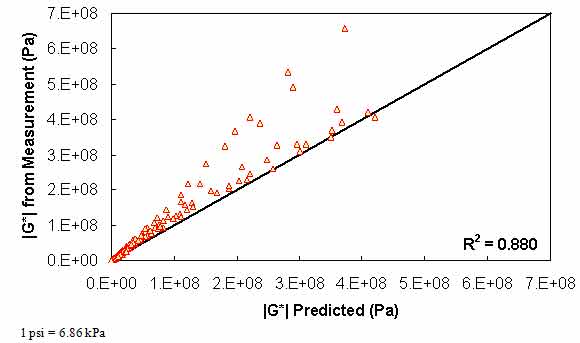
Figure 123. Graph. Level 1b verification of limited data analysis procedure in arithmetic scale using average shift factor function model.
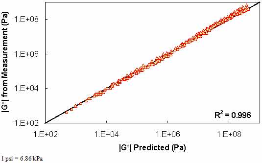
Figure 124. Graph. Level 1b verification of limited data analysis procedure in logarithmic scale using average shift factor function model.
Level 2 verification consists of data that have not been used in the development of either the PAR model or the t-T shift factor relationship. In addition, it consists of only DSR data, but the data cover the complete range expected in normal Superpave™ DSR characterization. A third level of verification that does not have the complete DSR data available is shown subsequently. The FHWA ALF study binders used previously to verify the PAR model are used for level 2 verification.
The steps taken in level 2 verification are as follows:
The major difference between level 1 and 2 verification is the lack of BBR data in the process. Because it is shown earlier in this section that differences in |G*| mastercurves can be large at temperatures below 41 °F (5 °C) when BBR data are not used for the calibration, only 41, 68, 105, and 129.2 °F (5, 20, 40, and 54 °C) data are used to analyze the differences in level 2 verification.
The results of level 2 verification are shown in figure 125 through figure 128. The model strength is good with an excellent coefficient of correlation. Both the average shift factor function and the phenomenological model show good results. The average function performs better in arithmetic space, and the phenomenological function appears to perform better in logarithmic space.
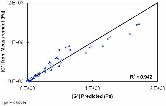
Figure 125. Graph. Level 2 verification of limited data analysis procedure in arithmetic scale using phenomenological shift factor function model.
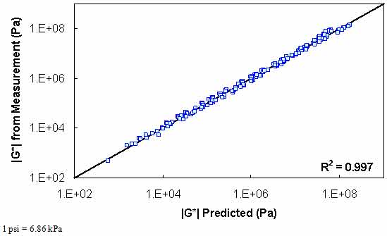
Figure 126. Graph. Level 2 verification of limited data analysis procedure in logarithmic scale using phenomenological shift factor function model.
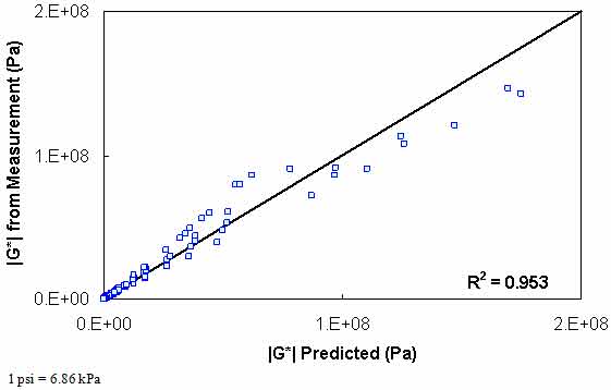
Figure 127. Graph. Level 2 verification of limited data analysis procedure in arithmetic scale using average shift factor function model.
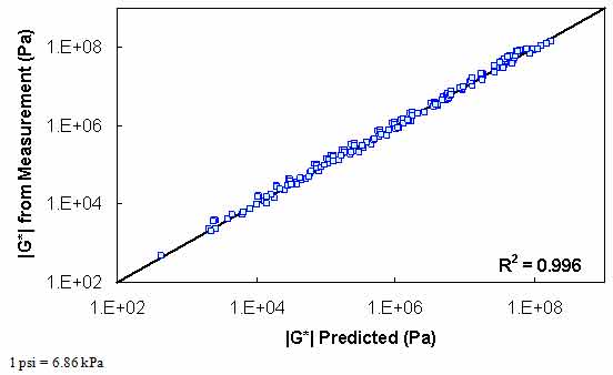
Figure 128. Graph. Level 2 verification of limited data analysis procedure in logarithmic scale using average shift factor function model.
The final verification level considered in this report is the verification of the analysis procedure for DSR data that are not complete. Specifically, the data at high temperatures are assumed to be unavailable. For this purpose, the FHWA mobile trailer database outlined in table 42 is used. As with level 2 verification, BBR data are unavailable for calibration purposes, and 14 °F (-10 °C) data are not included in the verification process. Without available high temperature data, it is assumed that each binder receives its high temperature grade based on the RTFO-aged binder (i.e., |G*|/sin(δ) = 0.32 psi (2.2 kPa) exactly at the high PG). In addition, it is known that asphalt binder has a phase angle of approximately 80 degrees at these high temperatures. These assumptions imply that |G*| at the high temperature PG is 0.31 psi (2,166 Pa), which is used in the fitting process.
The steps taken in level 3 verification are as follows:
The results of level 3 verification are shown in figure 129 through FIGURE 132. From these figures, it is observed that this dataset shows a reduction in predictability compared to the level 2 analysis but improved predictability as measured by R2. However, it should be noted that level 3 analysis does not include model data at 14 °F (-10 °C), while the two level 1 verification analyses do include these 14 °F (-10 °C) data.
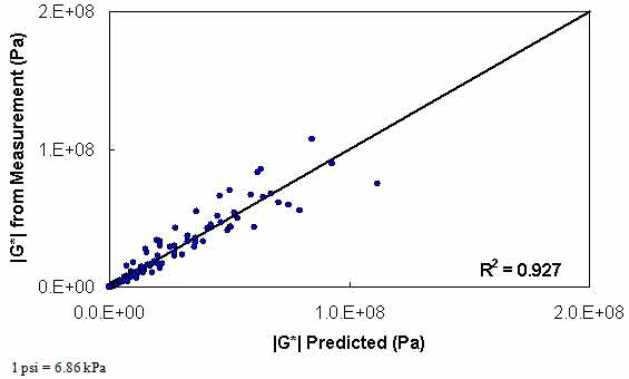
Figure 129. Graph. Level 3 verification of limited data analysis procedure in arithmetic scale using phenomenological shift factor function model.
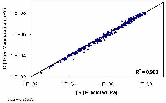
Figure 130. Graph. Level 3 verification of limited data analysis procedure in logarithmic scale using phenomenological shift factor function model.
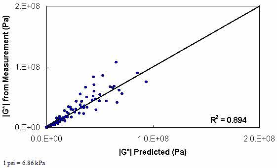
Figure 131. Graph. Level 3 verification of limited data analysis procedure in arithmetic scale using average shift factor function model.
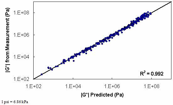
Figure 132. Graph. Level 3 verification of limited data analysis procedure in logarithmic scale using average shift factor function model.

