LTPP Computed Parameter: Dynamic Modulus

APPENDIX E: ANNACAP SOFTWARE MANUAL

E.1 INTRODUCTION

The Artificial Neural Networks for Asphalt Concrete Dynamic Modulus Prediction (ANNACAP) program has been developed under Contract No. DTFH61–02–00139 Task Order #10 LTPP Computed Parameter Dynamic Modulus to aid in populating the LTPP database with dynamic modulus data. Technical details concerning the analysis used in this program can be found in the final report for the referenced project. The purpose of this document is to provide a manual of operation for the ANNACAP program.

The dynamic modulus, |E*|, is a fundamental property that defines the stiffness characteristic of hot mix asphalt (HMA) mixtures as a function of loading rate and temperature. The significance of this material property is threefold. First, it is one of the primary material property inputs in the Mechanistic–Empirical Pavement Design Guide (MEPDG) and software developed by NCHRP Project 1-37A. The MEPDG uses mastercurves and time–temperature shift factors in its internal computations. The mastercurve is constructed using a hierarchical structure of inputs ranging from laboratory tests on HMA mixtures and binders to estimates based on properties of the HMA mixtures. Second, the |E*| is one of the primary HMA properties measured in the Superpave™ simple performance test protocol that complements the volumetric mix design. Third, |E*| is one of the fundamental linear viscoelastic (LVE) material properties that can be used in advanced HMA and pavement models that are based on viscoelasticity.

In spite of the demonstrated significance of |E*|, it is not included in the current LTPP materials tables because the database structure was established long before |E*| was identified as the main HMA property in the MEPDG. It is not practical to perform MEPDG level 1 laboratory |E*| tests on material samples from LTPP test sections at this time due to a lack of materials, budget limitations, and the absence of a suitable test method applicable to field samples obtained from relatively thin pavement structures. However, the LTPP database does contain other data that can be used to estimate the |E*| mastercurve and associated shift factors, estimate the |E*| at specific load durations and temperatures, or develop inputs to the models contained in MEPDG.

E.2 DISCLAIMER

This software is provided “as is,” and any express or implied warranties, including but not limited to the implied warranties of merchantability and fitness for a particular purpose, are disclaimed. In no event shall the authors be liable for any direct, indirect, incidental, special, exemplary, or consequential damages (including, but not limited to, procurement of substitute goods or services; loss of use, data, or profits; or business interruption) however caused and in any way theory of liability, whether in contract, strict liability, or tort (including negligence or otherwise) arising in any way out of the use of this software, even if advised of the possibility of such damage.

E.3 INSTALLATION INSTRUCTIONS

1. Insert ANNACAP Installation CD into the CD ROM or download zipped installer file from Web site. Note: If downloading the file, remember the location where you have unzipped the files.
2. If the CD does not autorun, press the Windows Start button.
3. Click on Run.
4. Change the directory to the location of the installer file (either the CD ROM drive or the unzipped file locations.
5. Select the Setup program.
6. Press OK.
7. Follow the onscreen instructions.
8. ANNACAP and all necessary support files will be installed.
9. A shortcut will be placed in the start menu under the Programs ⇒ ANNACAP path. To place a shortcut onto the desktop, users must manually perform the operation.

E.4 USING ANNACAP

E.4.1 Program Main Screen

The main ANNACAP screen is shown in figure 205. This screen appears when ANNACAP is launched. All analysis is menu–driven, and the menu schematic is shown in figure 206. To perform modulus predictions, users must provide the necessary inputs by following the File ⇒ Input path (described in detail below). Users must also provide a directory for output to be written by following the File ⇒ Output Directory path. Once both have been properly input, users may perform data analysis by following the File ⇒ Run Analysis path. Users may access this document by following the Help ⇒ Manual path or find basic program information by choosing the Help ⇒ About path.

Figure 205. Screenshot. ANNACAP main screen.

Figure 206. Illustration. ANNACAP menu diagram.

E.4.2 Input Data

Selecting the File ⇒ Input path will automatically launch the input utility. The initial screen shot is shown in figure 207. Users have four modes to choose from: (1) M_R-based ANN, (2) |G*|–based ANN, (3) viscosity–based ANN, and (4) batch mode. The screen is divided into two regions referred to as the left side and right side and separated by bordered regions. On the left side are areas for inputting basic information for the nonbatch mode runs, choosing the mode to use, and choosing the input parameter complexity to use. On the right side are inputs specific to the chosen analysis mode. Necessary inputs will appear on both the left and right sides of the screen as users make selections. After selecting all of the appropriate factors and entering all necessary inputs, pressing “Done” on the menu bar will return users to the main ANNACAP screen. Note that all modes will produce |E*| predictions at 14, 40, 70, 100, and 130 °F (-10, 4.4, 21.1, 37.8, 54.4 °C) and 25, 10, 5, 1, 0.5, and 0.1 Hz.

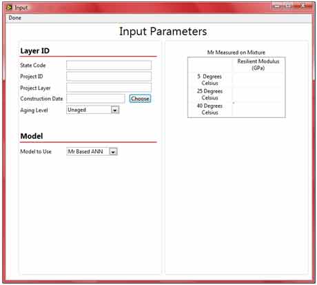
Figure 207. Screenshot. ANNACAP input screen.

E.4.3 Layer ID

Under the Layer ID section, users should enter the following items:

• State code.
• Project ID.
• Project layer.
• Construction date.
• Aging level (only RTFO aging is available for certain models).
• Test date (only if “Other” aging level is chosen).

The naming convention for these items is the same as that followed in the LTPP database. Users may choose to enter the dates directly into the appropriate boxes and, if they do so, the format should be Day–Abbreviated Month–Year (i.e., 20–Mar–1985). Users wishing to use the calendar utility should press the Choose button beside the date box and navigate to the appropriate date. When the appropriate date is chosen, users must press the OK button.

E.4.4 M_R-Based ANN

Selecting M_R-based ANN from the model drop–down menu will allow users to develop |E*| predictions based on M_R inputs. On the right side of the screen, users must enter M_R values in gigapascals at three specific temperatures (41, 77, and 104 °F (5, 25, and 40 °C)) into the provided table. The appropriate input ranges for these values are as follows:

• 41° F (5 °C) = 4,938,970.10 to 696,224.65 psi (34.053 to 4.8003 GPa).
• 77 °F (25 °C) = 2,235,176.58 to 156,785.79 psi (15.411 to 1.0810 GPa).
• 104 °F (40 °C) = 995,495.52 to 54,954.80 psi (6.8637 to 0.3789 GPa).

Inputting values outside this range will cause ANNACAP to display a warning indicating that input values exceed the calibration range, but predictions will still be made. Users should also select the aging condition for the measured M_R values.

E.4.5 |G*|-Based ANN

Selecting |G*|-based ANN from the model drop–down menu will allow users to develop |E*| predictions based on |G*| inputs. There are three different levels of input complexity: level 1, level 2, and level 3. For each level, users should input the percentage of voids in mineral aggregate (VMA) and percentage of voids filled with asphalt (VFA) in addition to |G*| values. The appropriate ranges for these input variables are shown beside the input controls. For all input levels, ANNACAP will use the CAM model to generate a mastercurve of the data. Users may choose to force the CAM model to fit the data with a certain glassy modulus value by choosing Input from the Find G_g by drop–down menu. If Input is chosen, the default value is 145,037.74 psi (1 GPa), but users may change it to any desired value. If users choose Fitting from the Find G_g by drop–down menu, then the glassy modulus is treated as any other optimization parameter. If no data are available at extremely low temperatures (below 32 °F (0 °C)), users are recommended to choose Input and select a value between 145,037.74 and 1,450,377.38 psi (1 and 10 GPa). If for some reason a fitting error occurs with the provided input, the program will display a fitting error dialog and not allow users to predict |E*|. If the calculated |G*| is greater than 675,875.86 psi (4.66 x 10⁹ Pa) or less than 0.029 psi (202 Pa), a warning dialog will appear, but |E*| predictions will be performed.

E.4.5.1 Level 1

For level 1, users have access to complete |G*| values at multiple temperatures and frequencies. These values should be entered directly into the table that appears on the right side of the screen. Users may choose to create this data file in another application and load it into the table by using the Load button. The file should be a tab delimited text file with the same column format as the input table. The file should have column labels.

E.4.5.2 Level 2

For level 2, users have access to |G*| values and possibly BBR stiffness values at multiple temperatures (at least two above 114.8 °F (46 °C) and two below 114.8 °F (46°C)) but at the fixed frequency of 10 rad/s and load time of 60 s. All of the measured moduli values should be at a consistent aging level. The |G*| values are entered in units of kilopascals, whereas the S(t) values are entered in units of megapascals following convention. The temperature is always entered in degrees Celsius. Users should enter the values into the tables on the right side of the screen.

E.4.5.3 Level 3

For level 3, users have access to |G*| values and possibly BBR stiffness values at multiple temperatures (at least two above 114.8 °F (46 °C) and two below 114.8 °F (46 °C)) at a fixed frequency of 10 rad/s and load time of 60 s. The aging conditions are a mixture of RTFO and PAV. The units are the same as those used in level 2 input. In addition to entering these values, users should choose the high temperature Superpave™ PG for the binder from the High Temp PG drop–down menu. If this information is not known or cannot be determined, users may select Unknown from the drop–down menu. In Level 3 analysis, only the RTFO-aging conditions may be predicted.

E.4.6 Viscosity-Based ANN

Selecting Viscosity–based ANN from the model drop–down menu will allow users to develop |E*| predictions based on viscosity inputs. There are three different levels of input complexity: level 1, level 2, and level 3. For each level, users should input the VMA and VFA. The appropriate ranges for these input variables are shown beside the input controls. If the calculated viscosity is less than 199,000 cP (199 Pas), a warning dialog will appear, but |E*| predictions will be performed.

E.4.6.1 Level 1

In level 1, users enter A and VTS values directly into the right side of the screen.

E.4.6.2 Level 2

In level 2, users choose the types of viscosity measures available by selecting or deselecting the radio buttons on the left side of the screen. The available measures include: R&BT temperature, penetration, absolute viscosity, and kinematic viscosity. Selecting or deselecting these measures will make appropriate input tables or controls appear on the right side of the screen. Following standard convention, the R&BT temperature is given in degrees Fahrenheit, the penetration is given by the PEN number, the absolute viscosity is input in poise, and the kinematic viscosity is input in centistokes. If users select kinematic viscosity, then they must also enter the binder–specific gravity in the G_bcontrol. By default, ANNACAP inputs 1.03 for G_b. Users must input at least two measures of viscosity so that A and VTS can be computed.

E.4.6.3 Level 3

In level 3, users choose the binder grade. Typical values compiled during the NCHRP 1–37A project are available, and the binder grades can be either Superpave™ –based, viscosity–based (AC system only), or penetration–based. The binder grade–to–viscosity relationship is summarized in table 78.

Table 78. Relationship between binder purchase specification grade and A and VTS parameters.

E.5 BATCH MODE

In batch mode, users enter four different files for the four different aging levels: (1) unaged or original binder data file, (2) RTFO–aged binder file, (3) PAV–aged binder file, and (4) field–aged binder file. Each file must be a tab delimited text file in order for ANNACAP to read the file. The file should have a header. Even if no data are available for some aging conditions, a file name must be entered into the directory path on the right side. The formatting for the original–, RTFO–, and PAV–aged conditions, collectively referred to as the lab–aged files, is different than the formatting for the field–aged binder file. The formats for the two files are presented in table 79 and table 80. Users may also view the format by selecting either the Format for Lab-Aged File or Format for Field-Aged File buttons.

E.6 OUTPUT DIRECTORY

Following the File ⇒ Output Directory path will launch the output directory dialog, as seen in figure 208. If no output directory is chosen or if users would like to change the current output directory, they should press the browse folder button to the right of the directory path (circled in black in figure 208). When this button is pressed, the folder selection dialog will appear (see figure 209). Users should then navigate to the desired output folder and select the Current Folder button (circled in black in figure 209). When selected, users return to the output directory dialog screen. To keep the chosen directory, users should press OK to return to the main screen. If users do not choose to keep the directory, press Cancel.

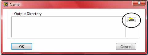
Figure 208. Screenshot. Output directory dialog.

Figure 209. Screenshot. Choosing output directory.

E.7 RUN ANALYSIS

To perform the dynamic modulus calculation, users should choose the File ⇒ Run Analysis path. The run analysis feature will become active only after ANNACAP has received valid input values. If an output directory has not been selected, an error message will appear, and the analysis will not be performed. Users must select a valid output directory and follow the File ⇒ Run Analysis path.

If users have chosen to follow either the M_R–based ANN, |G*|–based ANN, or viscosity–based ANN, a single output file with the quantities shown in table 81 will be generated and located in the output directory. The file name for this file will be Project_ID–Project_Layer–Aging Code–Model Type–Predicted Modulus.out. If users have chosen to follow the batch mode analysis technique, two different files will be generated: (1) a summary file with one row per layer and (2) a detailed output data file including 30 rows per layer (one row for each temperature and frequency combination). The summary analysis file for the batch mode will be formatted as shown in table 82. The file name for this file will be Models_Summary_Batch_Mode.out. The format for the main output file will be similar to that of the individual layer analysis and is shown in table 83. This file will be titled Predicted_Modulus_Batch_Mode.out. Both the summary and detailed output files will be located in the user–selected output directory. When running batch mode, users must rename the previous runs that are in the output directory because ANNACAP will overwrite existing file names without any warning to the user.

E.8 FORM OF SUPPLEMENTARY FUNCTIONS

E.8.1 CAM Model Function

(120)

Where:

(121)

Where:

E.9 TIME-TEMPERATURE SHIFT FACTOR FUNCTION FOR |G*|

E.9.1 Level 1 (WLF Function)

(122)

Where:

E.9.2 Levels 2 and 3

For the GV ANN models not using level 1 input, the shift factor is given by the following:

(123)

Where:

E.10 SIGMOIDAL FUNCTION

(124)

Where:

E.11 TIME-TEMPERATURE SHIFT FACTOR FUNCTION FOR |E*|

(125)

Where: