U.S. Department of Transportation
Federal Highway Administration
1200 New Jersey Avenue, SE
Washington, DC 20590
202-366-4000


Skip to content
Facebook iconYouTube iconTwitter iconFlickr iconLinkedInInstagram

Federal Highway Administration Research and Technology
Coordinating, Developing, and Delivering Highway Transportation Innovations

 
REPORT
This report is an archived publication and may contain dated technical, contact, and link information
Back to Publication List        
Publication Number:  FHWA-HRT-12-030    Date:  August 2012
Publication Number: FHWA-HRT-12-030
Date: August 2012


Estimation of Key PCC, Base, Subbase, and Pavement Engineering Properties From Routine Tests and Physical Characteristics

PDF Version (4.44 MB)

PDF files can be viewed with the Acrobat® Reader®

CHAPTER 5. MODEL DEVELOPMENT (6)

Table 21. Regression statistics for selected prediction model for 28-day PCC cylinder strength.

Variable

DF

Estimate

Standard Error

t-Value

Pr > |t|

VIF

Intercept

1

4028.41841

1681.71576

2.4

0.0215

0

w/c ratio

1

-3486.3501

2152.99857

-1.62

0.1134

2.40903

Cementitious content

1

4.02511

1.32664

3.03

0.0043

2.40903

The model statistics for table 21 are as follows:

Table 22. Range of data used for 28-day PCC cylinder strength.

Parameter

Minimum

Maximum

Average

w/c ratio

0.27

0.71

0.42

Cementitious content

376

936

664

Compressive strength

3,034

7,611

5,239


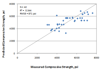
This graph shows an x-y scatter plot showing the predicted versus the measured values used in the 28-day cylinder compressive strength model. The x-axis shows the measured compressive strength from zero to 8,000 psi, and the y-axis shows the predicted compressive strength from zero to 8,000 psi. The plot contains 42 points, which correspond to the data points used in the model. The graph also shows a 45-degree line that represents the line of equality. The data are shown as solid diamonds, and they appear to demonstrate a good prediction. The measured values range from 3,034 to 7,611 psi. The graph also shows the model statistics as follows: N equals 42, R-squared equals 0.544 percent, and root mean square error equals 871 psi.

Figure 133. Graph. Predicted versus measured for 28-day cylinder compressive strength model.

This graph shows an x-y scatter plot showing the residual errors in the predictions of the 28-day cylinder compressive strength model. The x-axis shows the predicted compressive strength from zero to 8,000 psi, and the y-axis shows the residual compressive strength from zero to 2,500 psi. The points are plotted as solid diamonds, and they appear to show no significant bias (i.e., the data are well distributed about the zero-error line). There appears to be no trend in the data, and the trend line is almost horizontal (i.e., zero slope). The following equations appear in the graph: y equals -6E minus 0.7x plus 0.0014 and R-squared equals 5E minus 13.

Figure 134. Graph. Residual error plot for 28-day cylinder compressive strength model.

The recommended 28-day compressive strength model is as shown in figure 135.

f subscript c,28d equals 4,028.41841 minus 3,486.3501 times w/c plus 4.02511 times CMC.

Figure 135. Equation. Prediction model 1 for fc,28d.

Where:

f’c,28d= 28-day compressive strength, psi.

w/c = Water to cementitious materials ratio.

CMC = Cementitious materials content, lb/yd3.

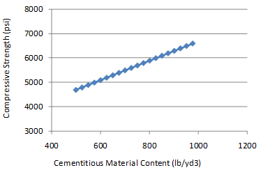
Figure 136 and figure 137 show the sensitivity of this model to w/c ratio and CMC. The change in compressive strength appears reasonable for both of the parameters for the range of values evaluated. They are also consistent with the data in the database. Within practical ranges, a change in CMC from 500 to 650 lb/ft3 increases the 28-day strength from approximately 4,700 to 5,300 psi for a w/c ratio of 0.4. Likewise, a decrease in the w/c ratio from 0.5 to 0.35 increases the strength from 4,700 to 5,200 psi.
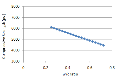
This graph shows the sensitivity of the 28-day compressive strength model to the water/cement (w/c) ratio. The x-axis shows the w/c ratio from zero to 0.8, and the y-axis shows the predicted compressive strength values from 3,000 to 8,000 psi. The sensitivity shown for w/c ratio ranges from 0.25 to 0.7, and the data are plotted using solid diamonds connected by a solid line. The graph shows that with increasing w/c ratio, the predicted compressive strength decreases.

Figure 136. Graph. 28-day compressive strength model sensitivity to w/c ratio.

This graph shows the sensitivity of the 28-day compressive strength model to the cementitious materials content (CMC). The x-axis shows CMC from 400 to 1,200 lb/yd3, and the y-axis shows the predicted compressive strength values from 3,000 to 8,000 psi. The sensitivity is shown for 
CMC ranges from 450 to 1,000 lb/yd3, and the data are plotted using solid diamonds connected by a solid line. The graph shows that with increasing CMC, the predicted compressive 
strength increases.

Figure 137. Graph. 28-day compressive strength model sensitivity to CMC.

Compressive Strength Model 2: Short-Term Cylinder Strength Model

Cylinder strength data were available for the SPS sections at pavement ages of 14 days, 28 days, and 1 year for a majority of the sections. Although two sections with strength data at 10 years were available, data in the model were limited for ages up to 1 year. Therefore, this model predicts the strength up to an age of 1 year.

Since this model utilizes only SPS data, a large set of independent variables was available for evaluation. Additionally, it is likely that this model will be used after approval of the mix design for a project or possibly even after initial construction, during which time more mix design parameters will be known for accurate prediction. The model developed includes pavement age as an independent parameter. Because the dataset includes multiple measurements or repeated readings of the same section, this parameter has been treated with a hierarchical modeling approach.


This model was established as shown in figure 138.

f subscript c,t equals 6,358.60655 plus 3.53012 times CMC minus 34.24312 times w/c times uw plus 633.3489 times natural log times open parenthesis t closed parenthesis.

Figure 138. Equation. Prediction model 2 for fc,t.

Where:

fc,t = Compressive strength at age t years, psi.

CMC = Cementitious materials content, lb/yd3.

w/c = Water to cement ratio.

uw = Unit weight, lb/ft3.

t = Short-term age, years.

The regression statistics for this model are presented in table 23, and details of the range of data used to develop the model are presented in table 24.

Table 23. Regression statistics for short-term cylinder strength model.

Variable

DF

Estimate

Standard Error

t-Value

Pr > |t|

VIF

Intercept

1

6,358.60655

1,213.09762

5.24

< 0 .0001

0

Cementitious

1

3.53012

0.90968

3.88

0.0002

2.15941

(w/c) × unit weight

1

-34.24312

11.00358

-3.11

0.0026

2.152

Ln(age)

1

633.3489

87.49625

7.24

< 0.0001

1.00604

The model statistics for table 23 are as follows:

Table 24. Range of data used for short-term cylinder strength model.

Parameter

Minimum

Maximum

Average

w/c ratio

0.27

0.69

0.43

Cementitious content

376

936

660

Unit weight

124

151

143

Pavement age

0.0384

1.0000

0.3081

Compressive strength

2,480

10,032

5,256

The model was developed using 79 data points, and the prediction has an R2 value of 66.6 percent and an RMSE value of 789 psi. The reason for an improved R2 compared to the 28-day strength model is not clear from these analyses. Figure 139 and figure 140 show the predicted versus measured plot and the residual plot, respectively.

This graph shows an x-y scatter plot showing the predicted versus the measured values used in the short-term cylinder compressive strength model. The x-axis shows the measured compressive strength from zero to 12,000 psi, and the y-axis shows the predicted compressive strength values from zero to 12,000 psi. The plot contains 79 points, which correspond to the data points used in the model. The graph also shows a 45-degree line that represents the line of equality. The data are shown as solid diamonds, and they appear to demonstrate a good prediction. The measured values range from 2,480 to 10,032 psi. The graph also shows the model statistics as follows: N equals 79, R-squared equals 0.666 percent, and root mean square error equals 789 psi.

Figure 139. Graph. Predicted versus measured for short-term cylinder compressive strength model.

This figure shows an x-y scatter plot showing the residual errors in the predictions of the short-term cylinder compressive strength model. The x-axis shows the predicted compressive strength from zero to 10,000 psi, and the y-axis shows the residual compressive strength from -3,000 to 3,000 psi. The points are plotted as solid diamonds, and they appear to show no significant bias (i.e., the data are well distributed about the zero-error line). There appears to be no trend in the data, and the trend line is almost horizontal (i.e., zero slope). The following equations are found in the graph: y equals 9E minus 0.7x minus 0.0082 and R-squared equals 2E minus 12.

Figure 140. Graph. Residual errors for short-term cylinder compressive strength model.


Federal Highway Administration | 1200 New Jersey Avenue, SE | Washington, DC 20590 | 202-366-4000
Turner-Fairbank Highway Research Center | 6300 Georgetown Pike | McLean, VA | 22101