Investigation of Increase in Roughness Due to Environmental Factors in Flexible Pavements Using Profile Data From Long-Term Pavement Performance Specific Pavement Studies 1 Experiment

CHAPTER 6. OVERALL ANALYSIS OF ROUGHNESS CHANGES AT SPS-1 TEST SECTIONS

This chapter presents the overall analysis of roughness changes at SPS-1 test sections, including the relationships between changes in MIRI and CLIRI, changes in IRI and structural strength, changes in IRI and subgrade type, changes in IRI and drainage, and changes in IRI and environmental conditions. This chapter also discusses the effect of PI of subgrade on changes in IRI, the relationship between changes in IRI and transverse cracking, and the effect of seasonal variations on IRI values. The chapter concludes with a detailed investigation of roughness increase at selected sections and a presentation of models for predicting the change in roughness due to environmental effects.

RELATIONSHIP BETWEEN CHANGES IN MIRI AND CLIRI

Figure 84 shows the relationship between the change in MIRI and the change in CLIRI for all SPS-1 test sections. The change in MIRI was greater than the change in CLIRI at 65 percent of the test sections. Figure 85 shows the relationship between the rate of change of MIRI and rate of change of CLIRI that were obtained from the regression analysis. The rate of change of MIRI was greater than the rate of change of CLIRI at 62 percent of the test sections.

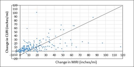
Figure 84. Graph. Change in CLIRI versus change in MIRI.

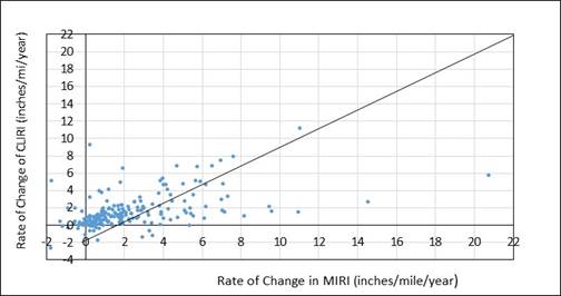
Figure 85. Graph. Rate of change of CLIRI versus rate of change of MIRI.

Figure 86 shows a box plot of the rate of change of MIRI and CLIRI. (See the first subsection of chapter 5 for a description of a box plot.) A rate of change of IRI greater than 10 inches/mi/year was noticed for MIRI at four sections and for CLIRI at one section. A rate of change of IRI less than −2 inches/mi/year was noticed for CLIRI at one section. These data points are not shown in figure 86 or any other plots included in this chapter because if these data points were shown in the plots, it would be difficult to see the changes that affect a majority of the sections. The median, first quartile, and third quartile values for rate of change of MIRI were 1.56, 0.55, and 3.22 inches/mi/year, respectively, while the corresponding values for CLIRI were 1.05, 0.31, and 1.19 inches/mi/year, respectively. A t-test indicated the mean value of MIRI was significantly greater than the mean value of CLIRI (significance level = 0.05, p-value = 0.002).

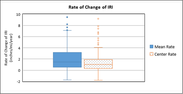
Figure 86. Graph. Box plots showing rate of change of MIRI and CLIRI.

RELATIONSHIP BETWEEN THE CHANGE IN IRI AND STRUCTURAL STRENGTH OF THE TEST SECTION

The relationship between the rate of change of MIRI and SN of the test sections is shown in Figure 87, while this relationship for CLIRI is shown in figure 88. A trend line fitted to each dataset using the method of least squares shows a clear trend of increasing rate of change of MIRI with decreasing SN, while for CLIRI, there was only a slight trend of increasing rate of change of CLIRI with decreasing SN.

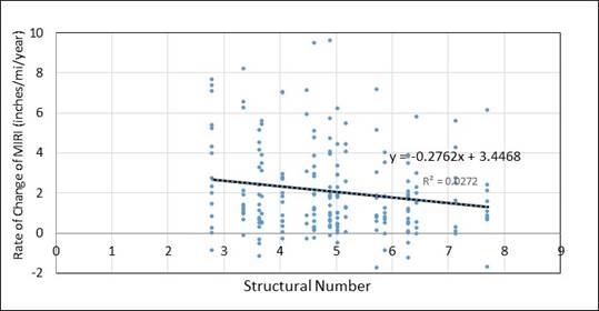
Figure 87. Graph. Relationship between rate of change of MIRI and SN of test sections.

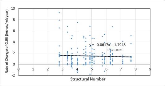
Figure 88. Graph. Relationship between rate of change of CLIRI and SN of test sections.

Test sections 7 and 13, with an SN of 2.8, were the structurally weakest test sections in the SPS‑1 experiment, while the next most structurally weak test sections in the SPS-1 experiment were test sections 2 and 20, with an SN of 3.36. For this analysis, test sections 2, 7, 13, and 20 were considered structurally weak test sections, and the other test sections were considered structurally strong test sections. Figure 89 shows a box plot of the rate of change of MIRI and CLIRI for the test sections that were categorized as weak and strong test sections. Table 90 summarizes the following information shown in figure 89 for each dataset: number of test sections; median, first quartile, and third quartile values for the rate of change of IRI; and the range of rate of change of IRI for each dataset excluding outliers. A t-test indicated the mean value of the rate of change of MIRI for weak sections was greater than that for the strong sections (significance level = 0.05, p-value = 0.039), and the mean value of rate of change of CLIRI for weak sections was greater than that for the strong sections (significance level = 0.05, p-value = 0.039).

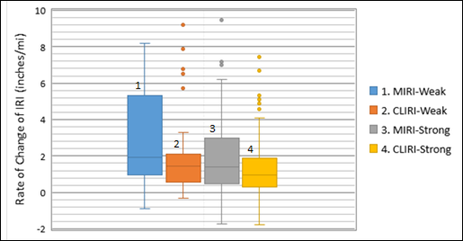
Figure 89. Graph. Box plots showing rate of change of MIRI and CLIRI for weak and strong sections.

Table 90. Median, first quartile, and third quartile values, and data ranges for rate of change of MIRI and CLIRI for weak and strong sections.

RELATIONSHIP BETWEEN CHANGES IN IRI AND SUBGRADE TYPE

Figure 90 shows a box plot of the rate of change of MIRI and CLIRI for the test sections based on the subgrade type (i.e., fine- and coarse-grained). Table 91 summarizes the following information shown in figure 90 for each dataset: number of test sections; median, first quartile, and third quartile values for the rate of change of IRI; and the range of rate of change of IRI for each dataset excluding outliers.

A t-test indicated the mean value of the rate of change of MIRI for sections on fine-grained subgrade was greater than that for section on coarse-grained subgrade (significance level = 0.05, p-value = 0.008), and the mean value of rate of change of CLIRI for sections on fine-grained subgrade was greater than that for sections on coarse-grained subgrade (significance level = 0.05, p-value < 0.001). The subgrade is expected to interact with precipitation and FI in affecting the change in IRI. The interaction between environmental conditions and subgrade type is examined later in this chapter in the subsection entitled Relationship Between Changes in IRI and Environmental Conditions.

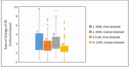
Figure 90. Graph. Box plots showing the rate of change of MIRI and CLIRI for sections on fine- and coarse-grained subgrades.

Table 91. Median, first quartile and third quartile values, and data ranges for rate of change of IRI for fine and coarse subgrades.

RELATIONSHIP BETWEEN CHANGES IN IRI AND DRAINAGE AT TEST SECTIONS

A PATB layer was present in the pavement structure to provide drainage at test sections 7 through 12 and 19 through 24. At sections 7 through 9 and 19 through 21, the PATB layer was located between the AC surface and the DGAB layer. In sections 10 through 12 and 22 through 24, the PATB layer was located between the ATB layer and the subgrade. Figure 91 shows a box plot of the rate of increase of MIRI for sections with and without drainage, categorized according to the subgrade type, while figure 92 shows a similar plot for the rate of increase of CLIRI.
Table 92 summarizes the following information shown in figure 91 and figure 92 for each dataset: number of test sections; median, first quartile, and third quartile values for the rate of change of IRI; and the range of rate of change of IRI for each dataset excluding outliers.

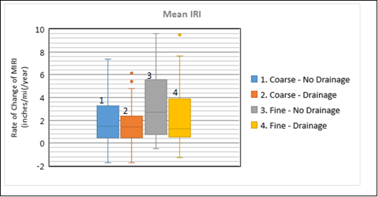
Figure 91. Graph. Box plots showing the rate of change of MIRI for sections with and without drainage, categorized according to subgrade type.

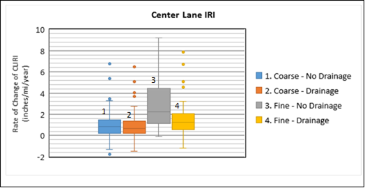
Figure 92. Graph. Box plots showing the rate of change of CLIRI for sections with and without drainage, categorized according to subgrade type.

Table 92. Median, first quartile, and third quartile values, and data ranges for rate of change of IRI for sections with and without drainage, categorized according to subgrade type.

The analysis showed the following:

• MIRI, Fine-Grained Subgrade: The median values of the rate of change of MIRI were 1.24 and 2.71 inches/mi/year for sections with and without drainage, respectively. The third quartile values of the rate of change of MIRI were 3.43 and 5.92 inches/mi/year for sections with and without drainage, respectively. A t-test indicated the mean value of the rate of change of MIRI for sections with and without drainage were not different (significance level = 0.05, p-value = 0.053). Note that the p-value was just over 0.05. However, overall, based on the third quartile value and the spread of the data, sections with drainage performed better in terms of the rate of change of IRI than sections without drainage.
  
  
• CLIRI, Fine-Grained Subgrade: The median values of the rate of change of CLIRI were 1.23 and 2.40 inches/mi/year for sections with and without drainage, respectively. The third quartile values of rate of change of CLIRI were 1.97 and 4.58 inches/mi/year for sections with and without drainage. A t-test indicated that the mean value of the rate of change of CLIRI for sections without drainage was greater than that for sections with drainage (significance level = 0.05, p-value = 0.011).
  
  
• MIRI, Coarse-Grained Subgrade: The median values of the rate of change of CLIRI were 1.40 and 1.55 inches/mi/year for sections with and without drainage, respectively. The third quartile values for the rate of change of MIRI for sections with and without drainage were 2.34 and 3.31 inches/mi/year, respectively. A t-test indicated that there was no difference in the mean value of the rate of change of MIRI for sections with and without drainage (significance level = 0.05, p-value = 0.30). However, overall, based on the third quartile value and the spread of the data, sections with drainage performed better in terms of the rate of change of IRI than sections without drainage.
  
  
• CLIRI, Coarse-Grained Subgrade: The median values of the rate of change of CLIRI for sections with and without drainage were 0.66 and 0.85 inches/mi/year, respectively. The third quartile values for the rate of change of CLIRI for sections with and without drainage were 1.36 and 1.46 inches/mi/year, respectively. A t-test indicated that there was no difference in the mean value of the rate of change of CLIRI for sections with and without drainage (significance level = 0.05, p-value = 0.44). The data shown in the box plots also did not show any clear difference in the rate of change of CLIRI for sections with and without drainage.

Overall, this analysis showed that the provision of drainage on test sections that had fine-grained subgrade reduced the rate of change of IRI. For sections on coarse-grained subgrade, sections with drainage overall showed a lower rate of change of MIRI, but there was no clear difference in the rate of change of CLIRI for sections with and without drainage. Note that subgrades categorized as coarse-grained subgrade would also have material finer than the No. 200 sieve, and drainage characteristics of pavements built on coarse-grained subgrades with a high content of fine material would be improved with the provision of drainage.

An evaluation was performed to determine what method of providing drainage (i.e., PATB over DGAB or PATB under ATB) resulted in a lower rate of change of roughness using the data from test sections constructed on fine-grained subgrade. Figure 93 shows a box plot for the rate of change of MIRI for sections on fine-grained subgrade categorized according to sections without drainage, sections with PATB over DGAB, and sections with PATB below the ATB. Figure 94 shows a similar plot for CLIRI. Table 93 summarizes the following information shown in figure 93 and figure 94 for each dataset: number of test sections; median, first quartile, and third quartile values for the rate of change of IRI; and the range of rate of change of IRI for each dataset excluding outliers.

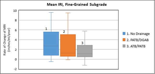
Figure 93. Graph. Box plots showing the rate of change of MIRI for sections on fine-grained subgrade, categorized according to type of drainage.

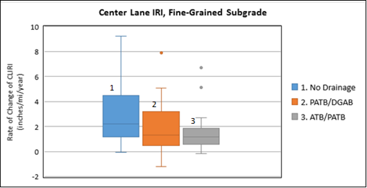
Figure 94. Graph. Box plots showing the rate of change of CLIRI for sections on fine-grained subgrade, categorized according to type of drainage.

Table 93. Median, first quartile and third quartile values, and data ranges for rate of change of IRI for sections on fine-grained subgrade, categorized according to the type of drainage.

The analysis showed the following:

• MIRI Values: A t-test indicated there was no difference in the mean value of rate of change of MIRI for sections with PATB over DGAB and ATB over PATB (significance level = 0.05, p-value = 0.11). The median value for the rate of change of MIRI for sections with no drainage, PATB over DGAB, and PATB below ATB were 2.72, 1.24, and 1.12 inches/mi/year, respectively. The third quartile values for the rate of change of MIRI for sections with no drainage, PATB over DGAB, and PATB below ATB were 5.92, 4.55, and 2.88 inches/mi/year, respectively. Although the t-test indicated there was no difference in the mean values for the rate of change of MIRI for sections with PATB over DGAB and PATB below ATB, the third quartile values showed that the sections with PATB below ATB performed better than the sections with PATB over DGAB.
  
  
• CLIRI Values: A t-test indicated there was no difference in the mean value of the rate of change of CLIRI for sections with PATB over DGAB and ATB over PATB (significance level = 0.05, p-value = 0.26). The median value for the rate of change of CLIRI for sections with no drainage, PATB over DGAB, and PATB below ATB were 2.40, 1.32, and 1.16 inches/mi, respectively. The third quartile values for the rate of change of MIRI for sections with no drainage, PATB over DGAB, and PATB below ATB were 4.58, 2.67, and 1.81 inches/mi/year, respectively. Although the t-test indicated there was no difference in the mean values for the rate of change of CLIRI for sections with PATB over DGAB and PATB below ATB, the third quartile values showed that the sections with PATB below ATB performed better than the sections with PATB over DGAB.

RELATIONSHIP BETWEEN CHANGES IN IRI AND ENVIRONMENTAL CONDITIONS

This subsection first categorizes the data used to analyze the relationship between changes in IRI and environmental conditions and discusses the results for changes in roughness for different environmental zones, interaction between environmental zone and subgrade type for roughness development, and interaction between provision of drainage and environmental zone.

Categorization of Data

Table 94 shows the SPS-1 projects categorized according to the environmental zone and subgrade type. In addition to the number of projects, this table also shows the number of SPS-1 test sections available in each category for analysis. As seen in table 94, the number of projects available in each category was not equal. For example, of the eight SPS-1 projects in the WNF zone, two projects were located on fine-grained subgrade, while six projects were located on coarse-grained subgrade. In the DNF zone, there were two projects, with one project located on fine-grained subgrade and the other located on coarse-grained subgrades. Only one SPS-1 project was constructed in the DF zone, and it was constructed on a coarse-grained subgrade. When comparing performance of test sections among the different environmental zones, there could be a bias because of unequal projects in each category. For cases where there were only one or two projects, the analysis could be heavily influenced by the poor performance of test sections in a specific project.

Table 94. SPS-1 projects classified according to subgrade type and environmental zone.

Changes in Roughness for Different Environmental Zones

Figure 95 and figure 96 show box plots for the rate of change of MIRI and CLIRI, respectively, classified according to the four environmental zones. Table 95 summarizes the following information shown in these two figures for each dataset: number of test sections; median, first quartile, and third quartile values for the rate of change of IRI; and the range of rate of change of IRI for each dataset excluding outliers.

For MIRI as well as CLIRI, the environmental zones in the order of increasing median values for the rate of change of IRI were WNF, DF, WF, and DNF. The number of SPS-1 projects that were located in the WNF, DF, WF, and DNF zones were eight, two, six, and two, respectively. The SPS-1 projects in the DNF zone were located in Arizona and New Mexico. All test sections in the New Mexico project had a relatively high rate of change of MIRI as well as CLIRI because of raveling. Hence, the high rate of change of MIRI and CLIRI for the DNF zone was not necessarily a reflection of the environment on pavement performance but was likely an AC mix related issue that caused the raveling.

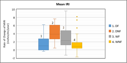
Figure 95. Graph. Box plots showing the rate of change of MIRI at SPS-1 sections according to environmental zone.

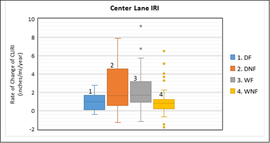
Figure 96. Graph. Box plots showing the rate of change of CLIRI at SPS-1 sections according to environmental zone.

Table 95. Median, first quartile, and third quartile values, and data ranges for rate of change of IRI for sections classified according to environmental zone.

A clear difference in the performance of test sections in the WF and WNF zones, which had six and eight projects, respectively, were observed in the data. The third quartile values for the rate of change of MIRI for the WF and WNF zones were 4.91 and 1.80 inches/mi/year, respectively, while the third quartile values for the rate of change of CLIRI for the WF and WNF zones were 3.01 and 1.23 inches/mi/year, respectively. A t-test also indicated that the mean values of MIRI as well as CLIRI for the WF region were greater than the corresponding values for the WNF zone (significance level = 0.05, p-value < 0.001).

Interaction Between Environmental Zone and Subgrade Type for Roughness Development

Of the eight SPS-1 projects in the WNF zone, two were located on fine-grained subgrade and six on coarse-grained subgrade. Of the six SPS-1 projects in the WF zone, four were located on fine-grained subgrade and two on coarse-grained subgrade. In the DNF zone, there was one SPS-1 project each located on fine- and coarse-grained subgrade, while both SPS-1 projects in the DF zone were located on coarse-grained subgrade. The change in IRI for the projects in the DNF, WF, and WNF zones classified according to subgrade type was examined to investigate the effect of subgrade type on the change in IRI.

The box plots in figure 97 and figure 98 show the rate of change of MIRI and CLIRI, respectively, classified according to subgrade type and environmental zone. Table 96 summarizes the following information shown in these two figures for each dataset: number of test sections, and median, first quartile, and third quartile values for the rate of change of IRI.

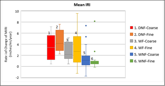
Figure 97. Graph. Box plots showing the rate of change of MIRI at sections in DNF, WNF, and WF zones, categorized according to subgrade type.

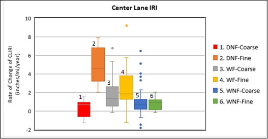
Figure 98. Graph. Box plots showing the rate of change of CLIRI for sections in DNF, WNF, and WF zones, categorized according to subgrade type.

Table 96. Median, first quartile and third quartile values, and data ranges for rate of change of IRI for sections classified according to environmental zone and subgrade type.

The analysis showed the following:

• DNF Zone: Overall, the box plots show the sections on fine-grained subgrade had a higher rate of change of IRI for MIRI as well as CLIRI when compared with sections on coarse-grained subgrade. In the fine-grained subgrade project, which was the New Mexico SPS-1 project, the MIRI as well as the CLIRI at test sections showed a high rate of change of IRI because of raveling of the AC surface. Hence, the differences in the changes between the sections on fine- and coarse-grained subgrade could not be attributed to the subgrade.
  
  
• WF Zone: A t-test indicated there was no difference in the mean values of the rate of change of MIRI as well as CLIRI for the two subgrade types in the WF zone. The third quartile values for the rate of change of MIRI for sections in the WF zone on coarse- and fine-grained subgrade were 4.42 and 5.47 inches/mi/year, respectively. For CLIRI, the third quartile values for the rate of change of CLIRI for sections in the WF zone that were on coarse- and fine-grained subgrade were 2.18 and 3.56 inches/mi/year, respectively. Based on these third quartile values, the sections on coarse-grained subgrade appear to have performed better than the sections on fine-grained subgrade with respect to the rate of change of IRI.
  
  
• WNF Zone: A t-test indicated there was no difference in the mean values of the rate of change of MIRI as well as CLIRI for the two subgrade types. The third quartile values for the rate of change of MIRI for sections on coarse- and fine-grained subgrade were 1.90and 0.96 inches/mi/year, respectively. The third quartile values for the rate of change of CLIRI for sections on coarse- and fine-grained subgrade were 1.26 and 1.15inches/mi/year, respectively. It was expected that the rate of change of IRI would be higher for sections on fine-grained subgrade. The two SPS-1 projects in the WNF zone located on fine-grained subgrade were in Alabama and Louisiana. The rate of change of MIRI as well as CLIRI for the Alabama project were very low, which resulted in low values being computed for the third quartile value for the rate of change of MIRI and CLIRI for sections on fine-grained subgrade.

Figure 99 shows the rate of change of CLIRI plotted versus the percent of subgrade passing through the No. 200 sieve for test sections in the WF zone. In this plot, the vertical series of data points shown for a specific value of percent material passing through the No. 200 sieve for the subgrade are for test sections in a specific SPS-1 project. A trend line fitted to the data shows that there was a weak trend of the rate of change of CLIRI increases with increasing fines content.

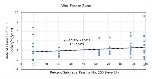
Figure 99. Graph. Rate of change of CLIRI versus percent subgrade passing through the No.200 sieve for SPS-1 sections in the WF zone.

Figure 100 shows the rate of change of CLIRI plotted versus the percent of subgrade passing through the No. 200 sieve for test sections in the WNF zone. A trend line fitted to the data shows that the rate of change of CLIRI did not appear to be influenced by the fines content in the subgrade.

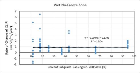
Figure 100. Graph. Rate of change of CLIRI versus percent material passing through the No. 200 sieve for SPS-1 sections in the WNF zone.

Interaction Between Provision of Drainage and Environmental Zone

Previously, a clear difference was observed in roughness progression rates for sections on fine-grained subgrade without drainage and drainage provided through a PATB layer incorporated into the pavement structure. The impact of drainage on test sections located on fine-grained subgrades in the different environmental zones was studied. Figure 101 and figure 102 show box plots of the rate of change of MIRI and CLIRI for sections with and without drainage located on fine-grained subgrade for different environmental zones. An SPS-1 project on fine-grained subgrade was not constructed in the DF zone; therefore, there is no data for the DF zone in these plots. The number of SPS-1 projects that were constructed on fine-grained subgrade in the DNF, WNF, and WF zones were one, two, and four, respectively. Table 97 summarizes the following information shown in figure 101 and figure 102 for each dataset: number of test sections and median, first quartile, and third quartile values for the rate of change of IRI.

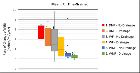
Figure 101. Graph. Box plots showing rate of change of MIRI for sections on fine-grained subgrade, categorized according to environmental zone and provision of drainage.

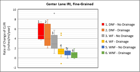
Figure 102. Graph. Box plots showing rate of change of CLIRI for sections on fine-grained subgrade, categorized according to environmental zone and provision of drainage.

Table 97. Median, first quartile, and third quartile values for rate of change of IRI for sections on fine-grained subgrade classified according to environmental zone and provision of drainage.

In each environmental zone, the median as well as the third quartile value for the rate of change of IRI for MIRI and CLIRI was higher for sections without drainage when compared with the sections with drainage.

Only one project was on fine-grained subgrade in the DNF zone—the project in New Mexico. As described previously in this report, all sections in that project had a high rate of change of IRI for MIRI as well as for CLIRI because of raveling of the AC surface.

The difference in the third quartile values for sections with and without drainage was highest for the WF zone for both MIRI and CLIRI, which indicated provision of drainage had a major impact on the rate of change of IRI for pavements constructed on fine-grained subgrades in the WF zone.

EFFECT OF PI OF SUBGRADE ON CHANGES IN IRI

The swelling potential of a fine-grained subgrade depends on the PI of the subgrade, with subgrades with higher PI values being more susceptible to swelling. Seven SPS-1 projects were located on fine-grained subgrade. The relationship between the PI of the subgrade and rate of change of MIRI and CLIRI for these projects was examined. Table 98 shows the SPS-1 projects constructed on fine-grained subgrade, the PI of the subgrade, and the median value of the rate of change of MIRI and CLIRI for the test sections in the project.

Table 98. SPS-1 projects constructed on fine-grained subgrade.

Figure 103 and figure 104 show the rate of change of MIRI and CLIRI, respectively, for all test sections in these projects plotted with the PI of the subgrade. The IRI values shown vertically for a specific value of PI are the IRI of the test sections contained within a specific SPS-1 project. A trend line fitted to the data points shows a trend of increasing rate of change of IRI with increasing PI values for both MIRI and CLIRI.

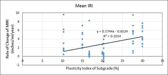
Figure 103. Graph. Rate of change of MIRI of test sections located on fine-grained subgrade versus the PI of the subgrade.

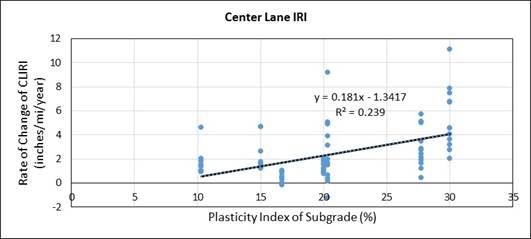
Figure 104. Graph. Rate of change of CLIRI of test sections located on fine-grained subgrade versus the PI of the subgrade.

RELATIONSHIP BETWEEN CHANGES IN IRI AND TRANSVERSE CRACKING

Von Quintus et. al. identified transverse cracking as a factor contributing to the increase in IRI of pavements and presented models for predicting the IRI of flexible pavements that included the total length of transverse cracks as an input to the model.⁽⁷⁾ The smoothness model for flexible pavements included in the AASHTO MEPDG software includes the total length of transverse cracking as a parameter for predicting the increase in IRI.⁽³⁾ In both of these models, the total length of transverse cracking within a section is summed up irrespective of the severity level of the transverse crack (i.e., low, medium, and high).

A transverse crack that extends across the center of the lane might affect CLIRI depending on the severity of the transverse crack. An analysis was performed to investigate the relationship between the change in CLIRI and the total length of transverse cracking at a section. The change in CLIRI at each section was computed by deducting the first CLIRI value from the last CLIRI value. Then, the distress survey date that was closest to the last date when IRI data were collected at the section was identified from the data in the MON DIS AC REV table in PPDB. Then, the total length of transverse cracking (i.e., all severity levels) corresponding to this date was summed for each test section. Figure 105 plots the change in CLIRI against the total length of transverse cracking within the section for all SPS-1 sections. The plot shows no relationship between these two parameters.

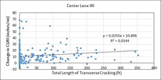
Figure 105. Graph. Relationship between the change in CLIRI and length of transverse cracking at test sections.

For a crack to affect CLIRI, that crack must extend across the center of the lane. Some of the transverse cracks located within a section might not have extended across the center of the lane. Such cracks would not have had an impact on CLIRI. Also, the impact of a crack on IRI was expected to depend on the severity level of the crack. Low severity level cracks might not have much of an impact on CLIRI. A crack would have a major impact on the IRI if there was a dip associated with the crack at the crack location. Such cracks are expected to be either medium or high severity level cracks. An example of how high severity level cracks that have a dip associated with the crack-affected CLIRI (SPS-1 section 300122) is described later in this chapter in the section entitled Detailed Investigation of Roughness Increase at Selected Sections.

THE EFFECT OF SEASONAL VARIATIONS ON IRI VALUES

Five SPS-1 test sections were part of the LTPP SMP program. These test sections were usually profiled four times a year to collect data during each season while the SMP program was in place. Table 99 shows the test sections that were in the SMP program and also indicates the climatic zone where the test section was located, the type of subgrade at the test section, and the percent material passing through the No. 200 sieve for subgrade.

Table 99. SPS-1 test sections that were in the seasonal monitoring program.

The two test sections in the Arizona SPS-1 project were profiled five times in 1998. Table 100 shows the CLIRI values obtained at these two test sections. At section 040113, CLIRI was 80 inches/mi for the first profile date, and thereafter the CLIRI values were between 85 and 89 inches/mi. It was not possible to identify the reason CLIRI at the first profile date was lower than the other CLIRI values by evaluating the profile data. At section 040114, the CLIRI values ranged from 50 to 53 inches/mi for the five profile dates, with this range being typically within the range of IRI associated with lateral wander during data collection. The CLIRI of these two sections located in the DNF region on a coarse-grained subgrade did not exhibit any seasonal effects.

Table 100. CLIRI values at section 040113 and 040114 in the Arizona SPS-1 project.

Figure 106 shows the CLIRI values over a 4-year period at section 300114 in the Montana SPS-1 project. Profile data at this site were collected five times a year in 2001, 2002, and 2003; three times a year in 2000; and four times a year in 2004. CLIRI over this period ranged from 45 to 49 inches/mi except on 8/16/2004 when CLIRI was 55 inches/mi. The variations in CLIRI between 45 to 49 inches/mi were typically within the range of IRI that could occur as a result of lateral variations in the profiled path. The reason for the higher CLIRI value on 8/16/2004 when compared with the other years could not be determined from the profile data. CLIRI values of this section, which was located in the DF region on a coarse-grained subgrade, did not exhibit any seasonal effects.

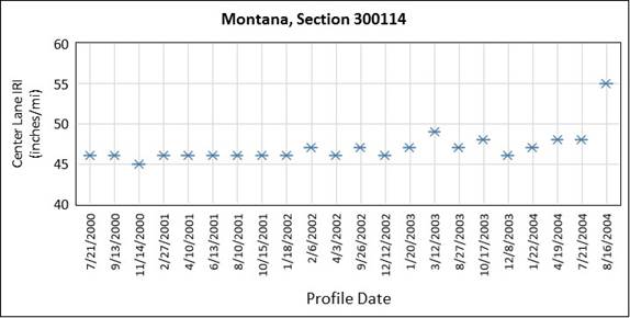
Figure 106. Graph. CLIRI values at section 300114 in Montana.

Section 320101 in the Nevada SPS-1 project was profiled five times a year in 1997, 2000, 2001, and 2002. Figure 107 shows the CLIRI values for the profile dates, which ranged from 50 to 52 inches/mi except for one occasion when CLIRI was 54 inches/mi. The CLIRI of this section, which was located in the DF region on a coarse-grained subgrade, did not appear to have been affected by any seasonal effects.

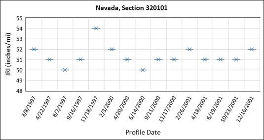
Figure 107. Graph. CLIRI values at section 320101 in Nevada.

Section 510114 in the Virginia SPS-1 project was profiled five times a year in 1998 and 2002 and four times a year in 2001 and 2003. Figure 108 shows the CLIRI values for the profile dates, which ranged from 63 to 66 inches/mi. This range is within the range of IRI typically expected as a result of lateral variations in the profiled path. The CLIRI of this section, which was located in the WNF region on a coarse-grained subgrade, did not appear to have been affected by any seasonal effects.

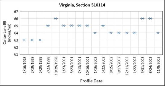
Figure 108. Graph. CLIRI values at section 510114 in Virginia.

For the test sections that were studied, which were all located on a coarse-grained subgrade and were situated in DF, DNF, and WNF environmental zones, the IRI values did not show any changes associated with seasonal influences.

DETAILED INVESTIGATION OF ROUGHNESS INCREASE AT SELECTED SECTIONS

The increase in CLIRI could be attributed to the change in the profile of the pavement that occurred as a result of environmental effects as well as cracks that traverse the center of the lane (i.e., transverse cracks) and cracking present along the center of the lane (i.e., block cracking and longitudinal cracking).

A detailed investigation of how roughness changes along the center of the lane was performed by evaluating the profile data collected at a select group of sections. One aim of this investigation was to see whether specific wavelengths that contributed to the increase in CLIRI could be identified. Test sections where no distresses were present as well as sections where cracking that could influence CLIRI was present were selected for this analysis.

Evaluation of Roughness Increases at Selected Sections

This subsection presents the results of evaluation of roughness increase on selected sections in New Mexico, Louisiana, Montana, Ohio, Arizona, and Oklahoma SPS-1 projects.

Section 350105

All sections in the New Mexico SPS-1 project showed a large change in CLIRI, with the average change in CLIRI of all sections in the New Mexico project being the highest of all SPS-1 projects. At section 350105 in the New Mexico SPS-1 project, CLIRI increased from 34 to 65 inches/mi from 3/11/1997 to 4/24/2006. The increase in MIRI during this period at this section was from 37 to 64 inches/mi. The distress survey that was performed on 3/28/2006 indicated that the section did not have any transverse or block cracking that could have affected CLIRI. The distress survey noted that approximately 40 percent of the surface was raveled. Figure 109 shows a continuous IRI plot (25-ft base length) for CLIRI from a profiler run performed on 3/11/1997 and 4/24/2006. This plot shows CLIRI increased throughout the section between these two dates. A PSD plot of the profile data shows the distribution of wavelengths in the profile. Figure 110 shows a PSD plot for these data collection runs and shows the increase in IRI occurred for all wavelengths less than 80 ft, and a specific range of wavelengths that contributed to the increase in IRI could not be identified. It appears that the raveling of the pavement was a major contributor to increasing CLIRI at this section.

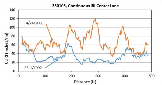
Figure 109. Graph. Continuous IRI plot showing the change in IRI along the center of the lane at section 350105.

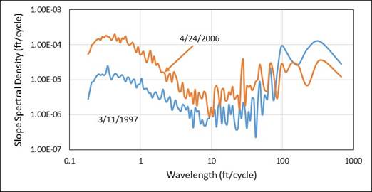
Figure 110. Graph. PSD plot for center of the lane data at section 350105.

Section 220114

At all sections, except for one, at the Louisiana SPS-1 project, the change in CLIRI was higher than the change in MIRI. At section 220114 in the Louisiana SPS-1 project, CLIRI increased from 31 to 52 inches/mi from 11/17/1997 to 1/16/2012. The increase in MIRI during this period at this section was from 40 to 48 inches/mi. The only distress recorded at this section at the last profile date was 85 ft of longitudinal nonwheelpath cracking that was of low severity; this cracking was located at the edge of the lane close to the inside lane. Hence, this cracking would not have had an impact on CLIRI. Figure 111 shows a continuous IRI plot for CLIRI (25-ft base length) from a profiler run that was collected on 11/17/1997 and 1/16/2012. This plot shows the IRI increased throughout the section between these two dates. Figure 112 shows a PSD plot of the data collected for these two dates, and the plot shows the increase in IRI occurred for most wavelengths, and a specific range of wavelengths that contributed to the increase in IRI could not be identified. The Louisiana SPS-1 project was on a fine-grained subgrade that had a PI of 20. Because there was no distress at this section, the increase in CLIRI appeared to have been caused by the change in the profile due to movement of subsurface layers (i.e., swelling or shrinkage of subgrade).

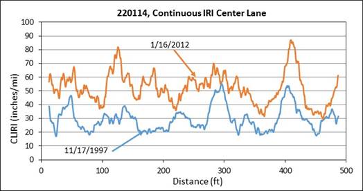
Figure 111. Graph. Continuous IRI plot showing the change in IRI along the center of the lane at section 220114.

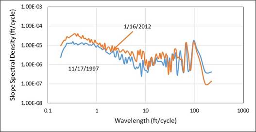
Figure 112. Graph. PSD plot for center of the lane data at section 220114.

Section 300122

At section 300122 in Montana, CLIRI increased from 47 to 77 inches/mi from 11/19/1998 to 7/17/2010. Figure 113 shows a plot of the center of the lane profile data collected at this section on 7/17/2010. Figure 114 shows a continuous IRI plot of CLIRI (25-ft base length) for the data collected on 11/19/1998 and 7/17/2010. The profile data plot shows there are three sharp downward features at 128, 247, and 465 ft, which are high severity transverse cracks, with a depression occurring adjacent to the cracks. The continuous CLIRI plot shows that a significant increase in CLIRI had occurred at the locations of these three transverse cracks between 11/19/1998 and 7/17/2010. In this section, the roughness associated with these three cracks was a major contributor to the increase in overall CLIRI of the section.

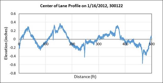
Figure 113. Graph. Center of the lane profile plot at section 300122.

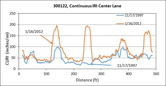
Figure 114. Graph. Continuous IRI plot showing the change in IRI along the center of the lane at section 300122.

Section 390112

Overall, only a few SPS-1 sections had block cracking, but many sections in the Ohio SPS-1 project had block cracking. Section 390112 had 43 percent of the area recorded as having high severity block cracking on the date closest to the last profile date. This block cracking was present along the center of the lane. CLIRI of section 390112 increased from 95 to 126 inches/mi from 11/12/1998 to 5/23/2012. Figure 115 shows a plot of the center of the lane profile data collected at this section on 5/23/2012 for one run, while figure 116 shows the continuous IRI plot of CLIRI (25-ft base length) for one run from the data collected on 11/12/1998 and 5/23/2012.

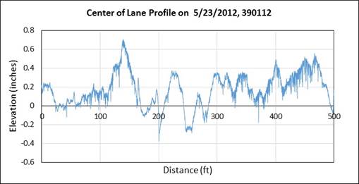
Figure 115. Graph. Center of the lane profile at section 390112.

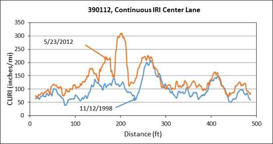
Figure 116. Graph. Continuous IRI plot showing the change in IRI along the center of the lane at section 390112.

The downward features in the profile plot represent the cracks associated with the block cracks that were present along the center of the lane. As seen from the continuous IRI plot, CLIRI of this section increased throughout the section from 11/12/1998 to 5/23/2012. A large increase in IRI is seen in the continuous IRI plot close to 200 ft, where a dip in the pavement was noted in the profile data. The block cracking that was present along the center of the lane was expected to have been a major contributor to the increase in CLIRI at this section.

Section 040119

CLIRI of section 040119 in the Arizona SPS-1 project increased from 49 to 62 inches/mi from 1/23/1997 to 3/27/2006. Figure 117 shows a plot of the center of the lane profile data collected at this section for the first run on 3/27/2006, while figure 118 shows a continuous IRI plot of CLIRI (25-ft base length) for the first data collection runs performed on 1/23/1997 and 3/27/2006. The profile plot shows some sharp downward spikes, which represent transverse cracks. The distress survey performed closest to the last profile date at this section indicated the section had 70 transverse cracks. The number of cracks with low, medium, and high severity were 50, 16, and 4, respectively. The total length of transverse cracks was 164 ft, and the distress maps showed several of these cracks traversed the center of the lane. No longitudinal cracking along the center of the lane or block cracking along the center of the lane that could have affected CLIRI was present at this section. The continuous IRI plot shows IRI had increased over a majority of the distance within the section from 1/23/1997 to 3/27/1996, with most of the increase in IRI occurring between 70 and 200 ft. No clear relationship between the transverse cracks in the profile plot and the increase in IRI from the continuous IRI plot could be observed.

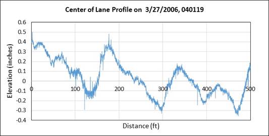
Figure 117. Graph. Center of the lane profile plot at section 040119.

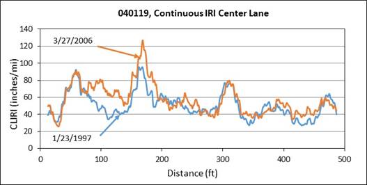
Figure 118. Graph. Continuous IRI plot showing the change in IRI along the center of the lane at section 040119.

Section 400121

CLIRI of section 400121 located in the Oklahoma SPS-1 project increased from 66 to 71 inches/mi from 11/19/1997 to 3/5/2011. The distress survey carried out on this section on the date closest to the last profile date indicated this section had 78 transverse cracks. The total length of the transverse cracks was 302 ft, with 97 percent of these transverse cracks classified as low severity. The distress survey map showed that several of these transverse cracks traversed the center of the lane. However, based on the increase in IRI, the transverse cracks do not seem to have had much of an effect on CLIRI.

Summary

Raveling of the AC surface contributed to the increase in IRI. Evaluation of the effect of low- and medium-severity cracks in increasing the IRI by studying profile plots and continuous IRI plots at a few sections did not show an increase in IRI that could be attributed to the cracking. The IRI computation algorithm includes a moving average meant to mimic tire enveloping, and a downward spike measured on a narrow crack will have little effect on the IRI because of the moving average applied to the profile data in the IRI algorithm before computing the IRI. Hence, a low or medium severity crack might not have much of an impact on the IRI. However, a deformation on the pavement associated with the crack, such as a depression on either side of the crack, could have a significant effect on increasing the IRI. It was also observed that high-severity block cracking would cause an increase in IRI.

MODELS FOR PREDICTING THE CHANGE IN ROUGHNESS DUE TO ENVIRONMENTAL EFFECTS

Figure 119 shows a box plot of the change in CLIRI that occurred at the test sections that were analyzed in this study classified according to the subgrade type (i.e., fine-grained or coarse- grained).

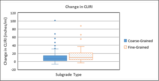
Figure 119. Graph. Box plots showing the change in CLIRI classified according to the subgrade type.

Figure 120 shows a box plot of the time period over which CLIRI values were obtained at the test sections classified according to the subgrade type. Figure 121 shows a box plot of the age of the pavement at the last profile date that was used for analysis. Table 101 through table 103 summarize the information shown in figure 119 through figure 121, respectively. The range of the data shown in these tables excludes outliers.

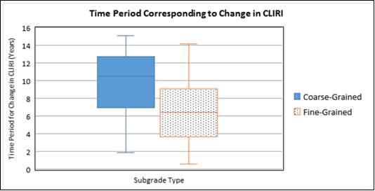
Figure 120. Graph. Box plots showing the period over which CLIRI was collected at the test sections, classified according to the subgrade type.

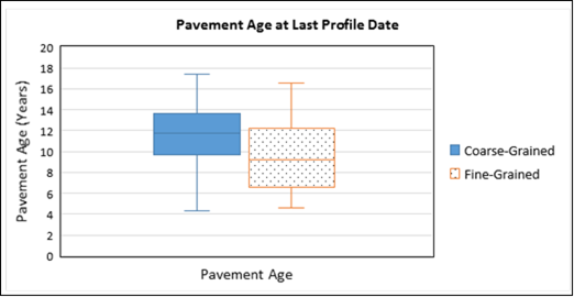
Figure 121. Graph. Box plots showing the age of the pavement at the last profile date used for analysis classified according to subgrade type.

Table 101. Median, first quartile, and third quartile values, and range of data for the change in CLIRI classified according to the subgrade type.

Table 102. Median, first quartile, and third quartile values, and range of data for the time
period over which CLIRI was obtained at test sections classified according to the subgrade type.

Table 103. Median, first quartile, and third quartile values, and range of data for the
pavement age at last profile date classified according to the subgrade type.

As shown in table 101, the median values for the change in CLIRI for sections on coarse- and fine-grained subgrade were 6.5 and 9.9 inches/mi, with the third quartile values for the change in CLIRI values for sections on coarse- and fine-grained subgrade being 14.1 and 20.6 inches/mi, respectively. The median value of the change in CLIRI for sections on both coarse- and fine-grained subgrade was not large, and therefore, developing models capable of predicting small changes in CLIRI could be very challenging.

The environmental parameters that could influence the increase in IRI were annual precipitation and FI. The subgrade parameters that could influence the increase in IRI were the percentage of subgrade passing through the No. 200 sieve (fines content) and the PI of the subgrade. Freezing would cause frost heave that could increase the IRI, while the PI of the subgrade would influence the swelling potential of the subgrade. Provision of a drainage layer was also a factor that affected the rate of change of IRI.

A model for predicting the change in CLIRI was first developed using linear regression by using all of the available data (i.e., sections on fine-grained and coarse-grained subgrade). Thereafter, separate models were developed for predicting the change in CLIRI for pavements on coarse- and fine-grained subgrade. Different combinations of the previously mentioned parameters were used to obtain the maximum R² value.

The model developed considering all data is shown in figure 122.

Figure 122. Equation. Formula for model developed for predicting the change in CLIRI considering all data.

Where:

ΔCLIRI = change in center of the lane IRI, inches/mi
Elapsed Time = period corresponding to the change in CLIRI, years
Precip = average annual precipitation, inches
P200 = subgrade passing the No. 200 sieve, percentage
FI = average annual FI, °F days/year

For the model in figure 122, R² equals 0.43, standard error equals 14.9 inches/mi, and the number of data points equals 201.

The model developed considering sections on coarse-grained subgrade is shown in figure 123.

Figure 123. Equation. Formula for model developed considering data for sections on coarse-grained subgrade.

For the model in figure 123, R² equals 0.37, standard error equals 14.2 inches/mi, and the number of data points equals 125.

The model developed considering sections on fine-grained subgrade is shown in figure 124.

Figure 124. Equation. Formula for model developed considering data for sections on fine-grained subgrade.

For the model in figure 124, R² equals 0.48, standard error equals 16 inches/mi, and the number of data points equals 76.

In all of these models, the R² values were low, and the standard error values were relatively high. Therefore, the change in CLIRI predicted by the models due to environmental effects can have a significant error. Including the total length of transverse cracking in the regression analysis did not result in a noticeable improvement in R² or a reduction in the standard error for all models.

The environmental parameters (i.e., precipitation and FI) for all test sections within an SPS-1 project are the same. The subgrade parameters (i.e., passing No. 200 and PI) for all test sections within a specific SPS-1 project were not available. Therefore, an average value for these parameters was computed by averaging the values that were available at the test sections that had data to compute an average value for the SPS-1 project. (See the subsection in chapter 4 entitled Subgrade Information for SPS-1 Projects.) This average value was assigned for all test sections in the project for the regression analysis. As shown in chapter 5, the change in CLIRI was different for different test sections in an SPS-1 project. However, although CLIRI for test sections in a specific project was different, in the regression analysis, the subgrade and environmental parameters for all test sections in an SPS-1 project were assumed to be the same. Therefore, for a specific SPS-1 project, the same set of parameters was being associated with different CLIRI values. This is likely one reason the standard error of the models shown in figure 122 through figure 124 are high and the R² values are low.