U.S. Department of Transportation
Federal Highway Administration
1200 New Jersey Avenue, SE
Washington, DC 20590
202-366-4000
Federal Highway Administration Research and Technology
Coordinating, Developing, and Delivering Highway Transportation Innovations
| REPORT |
| This report is an archived publication and may contain dated technical, contact, and link information |
|
| Publication Number: FHWA-HRT-16-045 Date: October 2016 |
Publication Number: FHWA-HRT-16-045 Date: October 2016 |
As previously stated, the objective of this research is to determine if the equation described in figure 1 can be used for conditions beyond those for which it is currently limited. The pier scour equations are evaluated using the scour observations from the field and laboratory datasets. The evaluation will compare the performance of the equations on data within the ranges specified in HEC-18 as well as beyond those ranges.
Performance is assessed by visual inspection of graphs of predicted and measured scour and by quantitative measures of reliability and accuracy. Reliability is defined by the reliability index (RI), which measures the risk of underpredicting the actual value of some property, which, in this case, is scour depth. A higher RI indicates a lower risk of underpredicting scour depth. RI is defined in general terms in figure 6.

Figure 6. Equation. RI.
Where:
Mx = Mean of a set of x values (dimension is that of the x values).
Sx = Standard deviation of a set of x values (dimension is that of the x values).
For this analysis, x is defined as shown in figure 7.
![]()
Figure 7. Equation. Ratio of measured to predicted scour depth.
Where:
x = Ratio of measured to predicted scour depth, dimensionless.
ys,m = Measured scour depth, ft (m).
ys,p = Predicted scour depth, ft (m).
To facilitate direct comparison between the laboratory and field data, accuracy is characterized by the relative error (RE) and the relative root mean square error (RRMSE). RE is defined in figure 8, and RRMSE is defined in figure 9.
![]()
Figure 8. Equation. RE.

Figure 9. Equation. RRMSE.
Where:
n = Number of observations.
The equations for general pier scour (figure 3) and pier scour for coarse bed materials (figure 1) both employ the following adjustments described by HEC-18:
In addition, the general pier scour equation employs K3 as described in HEC-18.
Comparison between measured and predicted scour estimates will employ dimensionless scour depths so that field and laboratory data may be directly compared. The dimensionless scour depth is defined in figure 10.
![]()
Figure 10. Equation. Dimensionless scour depth.
Application of the HEC-18 general pier scour equation to the full dataset resulted in predicted scour estimates that were compared to measured scour estimates in figure 11. Because the HEC‑18 equation is intended for design, it is not surprising that predicted scour is predominately greater than measured scour. A limited number of data points are not shown in the figure because the dimensionless predicted scour goes as high as 8.5.
Using the HEC-18 coarse bed material equation in the same manner results in the comparison summarized in figure 12. As a design equation, it also generally estimates scour depths exceeding measured values, though the patterns are not identical. For example, this equation results in a larger number of underpredicted scour values. As before, a limited number of data points are not shown in the figure because the dimensionless predicted scour for this equation goes as high as 10.2.
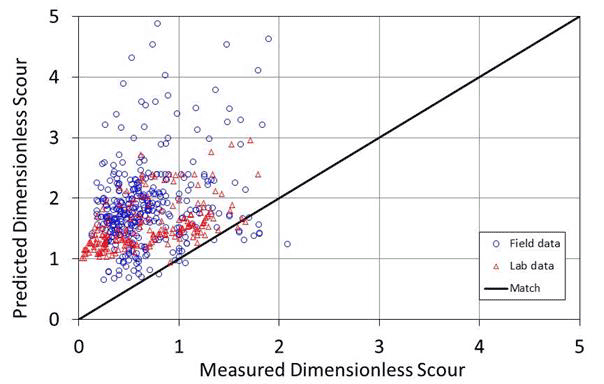
Figure 11. Graph. Predicted versus measured scour: HEC-18 general pier scour equation.
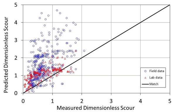
Figure 12. Graph. Predicted versus measured scour: HEC-18 coarse bed pier scour equation.
Table 4 provides detailed information on the performance of the HEC-18 general pier scour equation. The reliability of the equation reflected in the RI and the accuracy of the equation reflected in the RRMSE are provided for the data as a whole and partitioned into various groups. Results for the field and laboratory data are also differentiated.
| Data Description | HEC-18 Coarse Bed Criteria | Bed Load Transport | Gradation | D50 ≥ 0.79Inches | ||||||
|---|---|---|---|---|---|---|---|---|---|---|
| Source | Parameter | All | Yes | No | Clear Water | Live Bed | Uniform | Nonuniform | Yes | No |
| Field | n | 402 | 120 | 282 | 218 | 184 | 31 | 371 | 168 | 234 |
| RI | 2.56 | 6.22 | 2.16 | 2.42 | 2.75 | 2.29 | 2.58 | 1.10 | 1.24 | |
| RRMSE | 3.42 | 4.28 | 2.98 | 3.56 | 3.25 | 2.95 | 3.46 | 1.92 | 3.02 | |
| Lab | n | 192 | 0 | 192 | 163 | 29 | 52 | 140 | 0 | 192 |
| RI | 2.25 | 0.00 | 2.25 | 2.40 | 2.12 | 1.72 | 2.56 | 0.00 | 2.25 | |
| RRMSE | 5.10 | 0.00 | 5.10 | 5.52 | 1.18 | 3.80 | 5.51 | 0.00 | 5.10 | |
| Total | n | 594 | 120 | 474 | 381 | 213 | 83 | 511 | 168 | 426 |
| RI | 2.46 | 6.22 | 2.20 | 2.41 | 2.68 | 1.93 | 2.58 | 1.10 | 1.54 | |
| RRMSE | 4.04 | 4.28 | 3.98 | 4.50 | 3.05 | 3.51 | 4.12 | 1.92 | 4.09 | |
1 inch = 25.4 mm.
The RI and RRMSE measures for the combined dataset of 594 scour observations are 2.46 and 4.04, respectively. In the columns labeled HEC-18 Coarse Bed Criteria, the data are partitioned as follows based on the criteria described in HEC-18 for use of the coarse bed equation:
When all three criteria are met, HEC-18 recommends that the coarse bed pier scour equation be used rather than the general pier scour equation. For the field data, the RI of the general pier scour equation is 6.22 for the 120 observations meeting the criteria as coarse bed materials, while it is only 2.16 for the 282 observations not meeting the criteria. These results show that the HEC‑18 general pier scour is more reliable when applied to data meeting the coarse bed material criteria than it is for data not meeting the criteria. However, the reverse is true in terms of accuracy where the equation is more accurate for data not meeting the criteria (RRMSE = 2.98) compared with data meeting the criteria (RRMSE = 4.28).
Table 4 also summarizes the data partitioned by nonuniform (σ 1.5) versus uniform gradations as well as by median grain size greater than or equal to 0.79 inches (20.1 mm). None of the laboratory observations included data with D50 greater than 0.79 inches (20.1 mm).
Table 5 provides the performance information for the HEC-18 coarse bed material equation. The RI and RRMSE measures for the combined dataset of 594 scour observations are 1.19 and 2.66, respectively. Compared to the general pier scour equation, the coarse bed material scour equation is less reliable (more prone to underpredicting) but more accurate (lower RRMSE). Both of these observations are apparent when comparing figure 11 with figure 12.
With respect to the HEC-18 coarse bed criteria, the HEC-18 coarse bed equation is significantly more accurate for the field data meeting the criteria (RRMSE = 1.60) than for those data not meeting the criteria (RRMSE = 2.94). However, it is also less reliable (RI = 0.88 versus RI = 1.34) when considering the field data only.
| Data Description | HEC-18 Coarse Bed Criteria | Bed Load Transport | Gradation | D50 ≥ 0.79Inches | ||||||
|---|---|---|---|---|---|---|---|---|---|---|
| Source | Parameter | All | Yes | No | Clear Water | Live Bed | Uniform | Nonuniform | Yes | No |
| Field | n | 402 | 120 | 282 | 218 | 184 | 31 | 371 | 168 | 234 |
| RI | 1.18 | 0.88 | 1.34 | 0.91 | 1.70 | 1.61 | 1.16 | 1.10 | 1.24 | |
| RRMSE | 2.61 | 1.60 | 2.94 | 2.05 | 3.16 | 2.59 | 2.62 | 1.92 | 3.02 | |
| Lab | n | 192 | 0 | 192 | 163 | 29 | 52 | 140 | 0 | 192 |
| RI | 1.23 | 0.00 | 1.23 | 1.38 | 0.66 | 0.75 | 1.51 | 0.00 | 1.23 | |
| RRMSE | 2.75 | 0.00 | 2.75 | 2.97 | 0.59 | 2.79 | 2.74 | 0.00 | 2.75 | |
| Total | n | 594 | 120 | 474 | 381 | 213 | 83 | 511 | 168 | 426 |
| RI | 1.19 | 0.88 | 1.30 | 1.06 | 1.58 | 1.03 | 1.22 | 1.10 | 1.23 | |
| RRMSE | 2.66 | 1.60 | 2.87 | 2.49 | 2.94 | 2.72 | 2.65 | 1.92 | 2.90 | |
1 inch = 25.4 mm.
Prediction errors for both equations were evaluated against a variety of variables to expose trends that might exist. Figure 13 and figure 14 display the RE versus the ratio of the approach velocity to the critical velocity for the general and coarse bed equations, respectively. For ratios less than 1, clear water conditions exist, while for ratios greater than 1, live bed conditions exist. There is no apparent trend in RE with increasing bed transport capacity for either equation. In fact, it appears that for both equations, the distinction between live bed and clear water is not meaningful. A few observations (6 for the general pier scour equation and 2 for the coarse bed pier scour equation) exhibited REs exceeding 14 and are not shown on the figures.
Figure 15 and figure 16 present the REs versus the ratio of approach depth to median grain size for the general and coarse bed equations, respectively. For the general equation, a trend of decreasing error with increases in the ratio seems apparent, especially if the observations with the greatest errors are removed. Conversely, for the coarse bed equation, a trend of increasing error with increases in the ratio seems apparent.
Figure 17 and figure 18 show RE versus the gradation coefficient. Again, there is no discernable pattern in the error distributions for either equation between uniform versus nonuniform gradations.
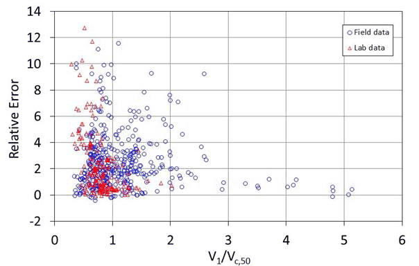
Figure 13. Graph. Error versus bed load transport: general equation.
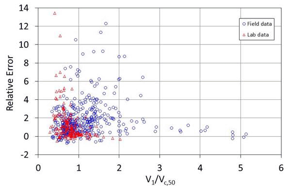
Figure 14. Graph. Error versus bed load transport: coarse bed equation.
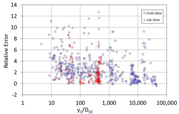
Figure 15. Graph. Error versus y1/D50: general equation.
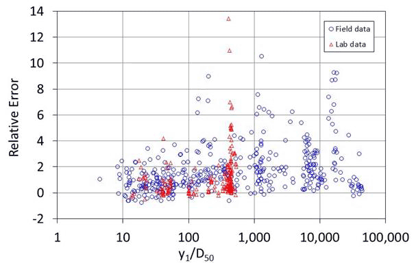
Figure 16. Graph. Error versus y1/D50: coarse bed equation.
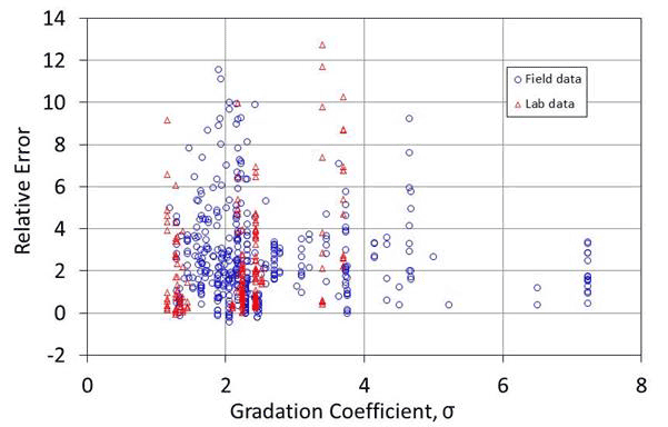
Figure 17. Graph. Error versus gradation coefficient: general equation.
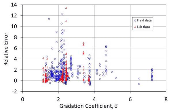
Figure 18. Graph. Error versus gradation coefficient: coarse bed equation.
For round nose piers aligned with the flow direction, HEC-18 recommends that predicted scour be limited to 2.4 times the pier width when the Fr is less than 0.8 and limited to 3.0 times the pier width when the Fr is greater than 0.8. These limits governed for 22 observations when using the general equation and for 20 observations when using the coarse bed equation. (Nine additional predicted scour estimates were limited by the wide pier adjustment when using both equations.)
The maximum measured dimensionless pier scour values were 2.6 in the field data and 1.8 in the laboratory data. Limiting the dimensionless predicted scour to 3.0 was evaluated relative to its effect on the RI and RRMSE. Such a limit only affects the field data because all predicted dimensionless scour values from both equations are less than 3.0 in the laboratory data. The results of this evaluation were mild increases in the accuracy and mild decreases in the reliability of both equations. Because development of such an adjustment was not an objective of this research, no further consideration was given. However, additional research into such a limit may be useful.
Bridge designers seek reliable (low risk of underdesign) and cost-effective (accurate) estimates of pier scour. Because a higher reliability generally means a lower accuracy, finding the most appropriate balance is a challenge. The trade-off is further complicated because although the study dataset is large and includes a wide variety of situations, it may not be representative for specific bridge design situations.
To address these challenges and to achieve the study objective, the coefficient from the HEC-18 coarse bed material equation (figure 1) was adjusted to a target RI. The selection of an appropriate target RI is best accomplished within the context of a larger risk analysis. For this study, it is noted that, for the general pier scour equation (figure 3) applied to the current dataset for the data not meeting the coarse bed criteria, the RI is 2.20 for 474 field and laboratory observations. For the coarse bed pier scour equation (figure 1), the RI is 0.88 for 120 field observations. Therefore, a target reliability of 2.0 is used that roughly reflects the composite reliability for pier scour estimates under current HEC-18 guidance.
To achieve an RI of 2.0 for the Hager number/gradation coefficient (HN/GC) based pier scour equation (figure 1), the coefficient required is 1.32. The resulting equation is shown in figure 19. Note that the adjustment for bed condition, K3, has been reintroduced to the HN/GC equation to evaluate its use for clear water (K3 = 1.1) and live bed (1.1 ≤ K3 ≤ 1.3) conditions. Because the previous analyses showed equivalent performance under a wide range of conditions, the equation is referred to as the HN/GC equation rather than as a coarse bed pier scour equation.
![]()
Figure 19. Equation. HN/GC equation for pier scour with RI = 2.0.
Application of the HN/GC pier scour equation to the full dataset results in predicted dimensionless scour estimates that are compared to measured dimensionless scour estimates in figure 20. Because the coefficient was increased, the predicted scour estimates also increased.
The maximum scour predictions using the equation were limited by the following:
For the HN/GC equation, the limits were enforced for 76 field observations and 9 laboratory observations.
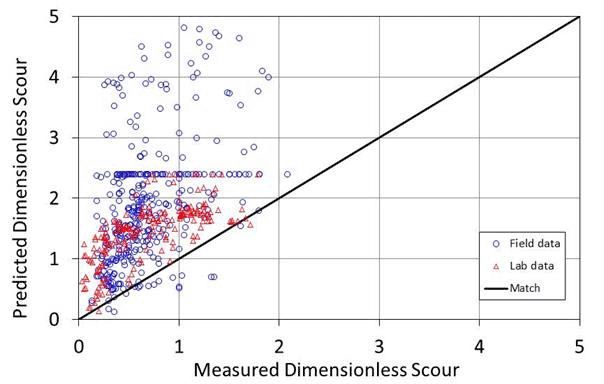
Figure 20. Graph. Predicted versus measured scour: HN/GC equation with RI = 2.0.
Table 6 provides the performance information for the HN/GC equation. The RI and RRMSE measures for the combined dataset of 594 scour observations are 2.0 (by design) and 3.67, respectively. The original development of the HN/GC equation was accomplished on a subset of the current dataset that generally (though not exclusively) met the requirements for application as the HEC-18 coarse bed equation. Therefore, when partitioning the data between those that meet the criteria and those that do not, it is not surprising that the equation is more accurate (lower RRMSE) for those data that meet the criteria. As shown in table 6, the RRMSE for data meeting the criteria is 2.34 while for the remaining data it is a much higher 3.94. However, because of the typical trade-off between accuracy and reliability, the equation is less reliable for the data meeting the criteria (RI=1.68) than for the data not meeting the criteria (RI = 2.12).
For the bed load partitioning, the same ambiguity between accuracy and reliability exists. The equation is more accurate in estimating clear water scour but more reliable in estimating live bed scour.
The gradation partition reveals virtually no distinction between uniform and nonuniform gradation. For the uniform and nonuniform partitions, the RIs are 2.01 and 2.02, respectively, and the RRMSEs are 3.75 and 3.66, respectively.
For D50, the picture is slightly different. The reliability is virtually identical between the two partitions: 1.96 for D50 ≥ 0.79 inches (20.1 mm) and 2.03 for D50 < 0.79 inches (20.1 mm). However, for the same level of reliability, the equation is more accurate for the larger D50 (RRMSE = 2.75) compared with the smaller D50 (RRMSE = 3.97).
| Data Description | HEC-18 Coarse Bed Criteria | Bed Load Transport | Gradation | D50 ≥ 0.79 Inches | ||||||
|---|---|---|---|---|---|---|---|---|---|---|
| Source | Parameter | All | Yes | No | Clear Water | Live Bed | Uniform | Nonuniform | Yes | No |
| Field | n | 402 | 120 | 282 | 218 | 184 | 31 | 371 | 168 | 234 |
| RI | 1.93 | 1.68 | 2.08 | 1.61 | 2.55 | 2.74 | 1.89 | 1.96 | 1.93 | |
| RRMSE | 3.61 | 2.34 | 4.03 | 2.87 | 4.32 | 3.62 | 3.60 | 2.75 | 4.11 | |
| Lab | n | 192 | 0 | 192 | 163 | 29 | 52 | 140 | 0 | 192 |
| RI | 2.24 | 0.00 | 2.24 | 2.40 | 2.00 | 1.65 | 2.60 | 0.00 | 2.24 | |
| RRMSE | 3.80 | 0.00 | 3.80 | 4.11 | 0.89 | 3.82 | 3.79 | 0.00 | 3.80 | |
| Total | n | 594 | 120 | 474 | 381 | 213 | 83 | 511 | 168 | 426 |
| RI | 2.00 | 1.68 | 2.12 | 1.85 | 2.49 | 2.01 | 2.02 | 1.96 | 2.03 | |
| RRMSE | 3.67 | 2.34 | 3.94 | 3.46 | 4.02 | 3.75 | 3.66 | 2.75 | 3.97 | |
1 inch = 25.4 mm.
Recall that the objective of this study is to determine if the equation described in figure 1 can be used for conditions beyond those to which it is currently limited. The previous observations suggest that the equation, modified with a revised coefficient to achieve a RI of 2.0, can be used for a broader range of conditions. These conditions are summarized as follows:
The HEC-18 pier scour methodology includes guidance to estimate scour for piers that are composed of groups of cylinders. Of the 402 field scour data observations, 60 involve pier groups. None of the laboratory observations include pier groups.
Table 7 provides the performance metrics for pier groups with the HN/GC equation from figure 19. The pier group observations show a significantly higher RI than for the single pier observations but with significantly lower accuracy. The HN/GC equation overpredicts all 60scour observations.
| Data Description | Pier Type | |||
|---|---|---|---|---|
| Source | Parameter | All | Group | Single |
| Field | n | 402 | 60 | 342 |
| RI | 1.93 | 3.36 | 1.81 | |
| RRMSE | 3.61 | 5.79 | 3.07 | |
Although the HN/GC could be used for pier groups, the addition of an adjustment factor reflecting pier groups might be appropriate. For the HN/GC equation, the factor would be less than one. It is recommended that this be investigated further for both this equation and the equation in figure 3. The 60 data observations in the current dataset could be used as a basis for further evaluation.