U.S. Department of Transportation
Federal Highway Administration
1200 New Jersey Avenue, SE
Washington, DC 20590
202-366-4000
Federal Highway Administration Research and Technology
Coordinating, Developing, and Delivering Highway Transportation Innovations
| REPORT |
| This report is an archived publication and may contain dated technical, contact, and link information |
|
| Publication Number: FHWA-HRT-16-023 Date: March 2016 |
Publication Number: FHWA-HRT-16-023 Date: March 2016 |
Prior to the field runs, speed harmonization algorithms were analyzed in micro-simulation environments. The simulation experiments examined various levels of CAV market penetration. Two speed harmonization algorithms were tested: speed-based and density-based. The speed-based algorithm was tested using Aimsun®, and the density-based algorithm was tested using INTEGRATION© and VISSIM®.
The speed-based algorithm determines advisory speeds for freeway segments upstream and downstream of a known bottleneck location based on measured speeds within the bottleneck area. The speed-based algorithm is intended to increase throughput and prevent bottleneck formation.
Within a bottleneck area, the speed-based algorithm tends to generate advisory speeds 10 to 50 percent higher than measured bottleneck speeds (see figure 4). Although the algorithm looks very simple, its function realizes the control philosophy in previous work.(8) This approach does not claim system optimization yet emphasizes simplicity and practical field implementation.
![]()
Figure 4. Equation. Speed-based algorithm speed advisory in bottleneck.
Where:
um(k) = Variable speed advisory at time step k in section m.
αm = Proportional
control gain in section m, where ![]() [1.1, 1.5]; default value: αm =
1.3.
[1.1, 1.5]; default value: αm =
1.3.
![]() = Measured speed of the bottleneck.
= Measured speed of the bottleneck.
Upstream of a bottleneck area, when traffic congestion approaches capacity levels, the speed-based algorithm tends to generate advisory speeds 10 to 30 percent below measured bottleneck speeds (see figure 5). Figure 5 shows that when bottleneck speed decreases, upstream advisory speed is proportionally reduced. This is equivalent to reducing flow to the bottleneck. When bottleneck speed increases, upstream advisory speed is proportionally increased. This increases bottleneck throughput towards its capacity.
![]()
Figure 5. Equation. Speed-based algorithm speed advisory upstream of bottleneck.
Where:
um + 1(k) = Variable speed advisory at time step k in section m + 1.
Vfree = Free-flow speed.
![]() = Measured occupancy
in bottleneck section.
= Measured occupancy
in bottleneck section.
Osw = Switch threshold of occupancy close to the capacity flow (suggested value is between 10.0 and 12.5 percent).
βm =
Proportional control gain in section m, where ![]() [0.7, 0.9]; default value: βm = 0.8.
[0.7, 0.9]; default value: βm = 0.8.
The speed-based speed harmonization algorithm streamlines traffic flow on each freeway segment. When there are multiple bottlenecks on a segment, advisory speeds for the segments between bottlenecks can be determined by distance-based interpolation.
To implement the advisory speeds for each freeway segment, CAVs are assumed to be discharged in platoons. The objective is for these vehicles to drive in parallel at the same speed on adjacent lanes in order to block all upstream vehicles. This forces all following vehicles to comply with the advisory speed.
Due to large variations in driver behavior on I-66, traffic speeds cannot be considered homogenous in both time and space. As a result, CAVs could use advisory speeds as set speeds but may not be able to drive at those speeds. Moreover, there would be speed differences between these CAVs on different lanes. When blocked by other vehicles in slow lanes, CAVs are expected to lag behind. Such situations have been observed in simulation. Therefore, it is necessary to adjust advisory speeds according to CAV speeds at a microscopic level. The following describes two methods of speed fusion tested through simulation: minimum group speed and average group speed.
Figure 6 implements an approach that uses the minimum speed of a group of research vehicles (i.e., the minimum group speed approach). First, the minimum speed among a group of CAVs is selected using lead vehicle speed in each lane. Then for each group and section that the group currently resides in, minimum speed is fused with global advisory speed (see figure 6). In essence, this fusion approach (based on market penetration rates) dictates that all CAVs must drive either at a similar speed or side-by-side.

Figure 6. Equation. Speed-based algorithm minimum group speed approach.
Where:
![]() = Variable speed advisory at time step k in section m for a typical group i of CAVs.
= Variable speed advisory at time step k in section m for a typical group i of CAVs.
Vimin(k) = Minimum measured speed at time step k for a typical group i of CAVs.
Figure 7 implements an approach that uses the average speed of a group of research vehicles (i.e., the average group speed approach). First, the average speed among a group of CAVs is estimated. If there is more than one vehicle in each lane, this is accomplished by selecting the average speed among leader vehicles in each lane. Then for each group and each section that the group currently resides in, average speed is fused with global advisory speed (see figure 7). In contrast with the minimum group speed approach, the average group speed approach dictates that CAVs do not need to drive side-by-side. They are allowed to have more speed differential within the same group but retain a close proximity, as determined by the weighting factors.
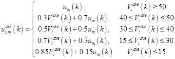
Figure 7. Equation. Speed-based algorithm average group speed approach.
Where:
![]() = Average measured
speed at time step k for a typical group i of CAVs.
= Average measured
speed at time step k for a typical group i of CAVs.
The speed-based algorithm was tested on the Aimsun® simulation platform. The results are presented in the following subsections.
Most default values for parameters such as time headway distribution and variance, maximum acceleration and variation, etc., were obtained from Performance Measurement System and Next Generation SIMulation data analyses. Two performance parameters were used to quantify the discrepancy between field-measured and simulated results in terms of throughput: relative root mean square error (RMSE) and the GEH statistic. Throughput comparisons were performed at all freeway mainline sensors, and speed comparisons were performed at three sensors.
An iterative calibration process was used. This process included progressive calibration at each sensor location from downstream to upstream and then in the reverse direction. This progressive calibration was necessary because upstream and downstream flows and speeds affect each other. The objective was to match both flows and time-mean speeds at fixed sensor locations. Minor demand adjustments were made to correct some sensor measurement errors, which were usually about 5 to 10 percent in practice. Engineering judgment was used to perform trial-and-error adjustments of both flows and speeds for upstream and downstream traffic situations. To obtain unbiased (i.e., "apples-to-apples") comparisons, it was important to confirm that all demand volumes were discharged at the end of each simulation run.
The proposed speed-based algorithm was simulated using the calibrated Aimsun® network for 3 virtual days with compliance rates of 10, 25, 50, and 100 percent. Each date was simulated for 10 replications (random number seeds) to get their mean. The following macroscopic performance measures were used to evaluate the algorithms' implementations within simulation: total travel time (TTT), total travel distance (TTD), total delay (TD) (obtained by deducting hypothetical free-flow travel times from simulated travel times), speed variation (directly reflects fluctuations in system-wide speed), total number of stops (TNOS) (used as a system-wide performance parameter for traffic smoothness in Aimsun®), and outflow (throughput) changes at bottlenecks.
CAV groups were regularly dispatched into the freeway segment from upstream of the I-66 and VA-267 merge. All CAVs were in ACC mode with fused speeds as set speeds, and all other vehicles were in human driver mode. Dispatching time intervals of 60, 90, 120, 900, and 1,800 s were used in simulation. In addition to the speed harmonization set speed, two other factors affected the practical speeds: downstream traffic and the speed of other vehicles in the group. Each lane had at least one CAV lane controlled through the Aimsun® application program interface.
Since the simulation model was set during the afternoon peak hours between 3 and 9 p.m., different random number seeds produced different demand flow patterns (from entrance ramp and freeway mainline), resulting in slightly different total (cumulative) demands. Higher total demands within any simulation time interval could result in longer TTT even if the speed harmonization algorithm was functioning properly. To overcome this bias, the following adjustments shown in figure 8 through figure 10 were applied when estimating percentage time improvements for TTT, TD, and TNOS. For example, if TTD increased by 10 percent after simulation, then TTT and TD were decreased by 10 percent as a penalty. Here the subscripts indicate whether parameters were estimated from the default scenario (default) or from data with speed control activated (vsa).
![]()
Figure 8. Equation. Speed-based algorithm TTT adjustment.
![]()
Figure 9. Equation. Speed-based algorithm TD adjustment.
![]()
Figure 10. Equation. Speed-based algorithm TNOS adjustment.
Table 1 shows that the system-wide performance measures when using the average group speed approach improved under faster dispatch rates. In a real-world field test, the fastest dispatching rates would be constrained by the total number of CAVs available and the time needed to finish a run cycle.
| CAV Dispatch Rate (s) | TTT (Percent) | TTD (Percent) | TD (Percent) | Speed Variation Percent) | Average Number of Stops (Percent) | Flow Downstream of Bottleneck (Percent) | Flow at Bottleneck (Percent) |
|---|---|---|---|---|---|---|---|
1,800 |
-0.63 | -0.04 | -1.84 | 0.19 | 0.070 | -0.18 | -0.41 |
900 |
-1.54 |
-0.03 |
-3.46 | -0.17 | 0.180 | 0.01 | -0.31 |
120 |
-4.08 |
0.52 |
-7.09 | -0.97 | 0.013 | 0.49 | -0.39 |
90 |
-4.45 |
0.66 |
-5.82 | -1.01 | -0.230 | 0.42 | -0.57 |
60 |
-6.53 |
0.87 |
-9.14 | -1.94 | 0.190 | 0.67 | -0.65 |
The objective of the density-based algorithm is to prevent upstream density from exceeding a critical density. The algorithm also tries to maximize bottleneck throughput by metering upstream flows. The algorithm searches for an optimal density that can maximize the bottleneck discharge rates while eliminating capacity drops. In the density-based algorithm, this optimal density is called the "target density."
Figure 11 illustrates a lane-drop bottleneck. The road section is divided into three zones: the speed harmonization zone, the acceleration zone, and the bottleneck. In order to develop a speed harmonization algorithm, three sets of sensors are placed: one in the speed harmonization zone, one directly upstream of the bottleneck, and one directly downstream of the bottleneck. If on- and/or off-ramps exist between the speed harmonization zone and the bottleneck, sensors are needed on the on- and off-ramps to record traffic flow. Sensors gather volume, speed, and occupancy data for use in the algorithm. CAVs in the speed harmonization zone receive advisory speed recommendations from a traffic management center to control flow arriving at the bottleneck.
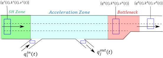
Figure 11. Illustration. Lane-drop bottleneck.
Where:
SH Zone = Speed harmonization zone.
qs(t) = Flow rate in the speed harmonization zone at time t.
ks(t) = Density of the speed harmonization zone at time t.
vs(t) = Speed in the speed harmonization zone at time t.
![]() = On-ramp flow rate at time t.
= On-ramp flow rate at time t.
![]() = Off-ramp flow at time t.
= Off-ramp flow at time t.
qu(t) = Capacity of the bottleneck zone at time t.
ku(t) = Density at capacity of the bottleneck zone at time t.
vu(t) = Speed in the bottleneck zone at time t.
qd(t) = Downstream capacity of the bottleneck at time t.
kd(t) = Downstream density at capacity of the bottleneck at time t.
vd(t) = Speed downstream of the bottleneck at time t.
The speed harmonization approach assumes that a steady-state fundamental diagram exists to relate the traffic stream flow (q), density (k), and speed (v) given the functions in figure 12 and figure 13.
![]()
Figure 12. Equation. Steady-state flow as a function of density.
Where:
Q(k) = General function Q of k based on a calibrated fundamental diagram.
![]()
Figure 13. Equation. Steady-state speed as a function of density.
Where:
V(k) = General function V of k based on a calibrated fundamental diagram.
Figure 14 shows the fundamental diagram for upstream and downstream sections of the bottleneck.
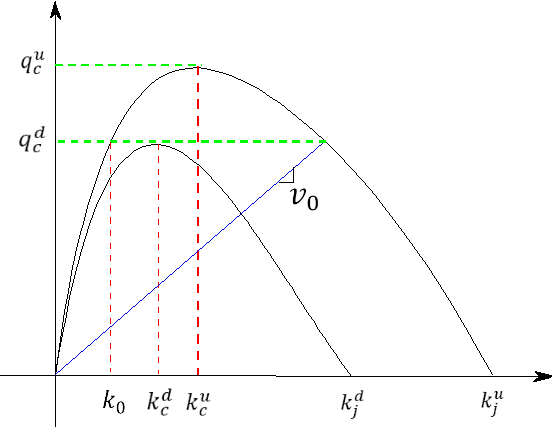
Figure 14. Illustration. Fundamental diagram of traffic flow.
Where:
quc = Capacity directly upstream of the bottleneck.
qdc = Downstream capacity of the bottleneck.
v0 = Advisory speed recommendation.
kdc= Downstream density at capacity of the bottleneck.
kuc= Density at capacity directly upstream of the bottleneck.
kdj= Downstream jam density of the bottleneck.
kuj= Jam density directly upstream of the bottleneck.
In order to avoid a traffic breakdown upstream of the bottleneck, arrivals are constrained at the bottleneck. Here, target density k0 (or its equivalent occupancy given that density cannot be measured in the field) is set in order to achieve the desired objective. The in-flow rate of the bottleneck at the capacity of the bottleneck is controlled.
The primary objective function of the speed harmonization algorithm is to maximize a weighted combination of flow downstream of the bottleneck and to minimize speed variability within the speed harmonization section, as shown in figure 15.

Subject to:
![]() ;
;
![]() ;
;
![]() ;
;
![]()
Figure 15. Equation. Mathematical formulation of the density-based algorithm.
Where:
v0(t) = Set of all possible advisory speed recommendations in the speed harmonization zone at time t.
T = Total simulation time.
wq = Weight assigned to the flow directly downstream of the bottleneck.
wv = Weight assigned to the speed variability in the speed harmonization zone.
![]() (t) = Measure of speed
variability in the speed harmonization zone (i.e., the standard deviation of
the speed in the speed harmonization zone at the control duration).
(t) = Measure of speed
variability in the speed harmonization zone (i.e., the standard deviation of
the speed in the speed harmonization zone at the control duration).
![]() = Flow rate at time t in speed harmonization zone.
= Flow rate at time t in speed harmonization zone.
qr(t) = Sum of flow rates at all on- and off-ramps between the speed harmonization zone and the bottleneck at instant t.
![]() = Difference between
speed advisory speed recommendations over the control interval in the speed
harmonization zone at time t.
= Difference between
speed advisory speed recommendations over the control interval in the speed
harmonization zone at time t.
![]() = Maximum allowed
change in control speed in the speed harmonization zone.
= Maximum allowed
change in control speed in the speed harmonization zone.
![]() = Advisory speed recommendation in the speed harmonization zone at time t.
= Advisory speed recommendation in the speed harmonization zone at time t.
vmin = Minimum advisory speed recommendation.
One criterion to determine when the speed harmonization should be activated can be expressed as kuc= k0. Also, qr(t) can be estimated using figure 16.
![]()
Figure 16. Equation. Estimation of flow rates.
Where:
ljout = Lag for vehicles traveling from speed harmonization zone to off-ramp j.
ljin Lag from speed harmonization zone to on-ramp i.
Lags are computed assuming that vehicles travel from the speed harmonization zone to given locations at the free-flow speed or, potentially, at the prevailing space-mean speed. In that sense, some form of prediction is needed to predict these flows.
![]() can be estimated to achieve optimal flow rates in the speed harmonization zone,
can be estimated to achieve optimal flow rates in the speed harmonization zone, ![]() . Reverse functions for flow-density and speed-density relationships under congested traffic can be defined to reflect the area upstream of the bottleneck as follows:
. Reverse functions for flow-density and speed-density relationships under congested traffic can be defined to reflect the area upstream of the bottleneck as follows:
![]()
Figure 17. Equation. Steady-state density as a reverse function of speed.
![]()
Figure 18. Equation. Steady-state density as a reverse function of flow.
Figure 19 illustrates a flowchart of the algorithm, which is described in the succeeding list.

Figure 19. Flowchart. Density-based algorithm logic and advisory speed recommendations.
1. When t < t0 (starting time when the algorithm is activated), assign the speed harmonization zone advisory speed recommendation, as shown in figure 20.
![]()
Figure 20. Equation. Density-based algorithm step 1—advisory speed recommendation.
Where:
vf = Free flow speed.
Optimal flow rate in the speed harmonization zone is set, as shown in figure 21.
![]()
Figure 21. Equation. Density-based algorithm step 1—optimal flow rate.
2. At each time step t, check the two conditions, as shown in figure 22.
![]()
Figure 22. Equation. Density-based algorithm step 2—flow and density conditions.
Where:
l = Time lag for vehicles traveling fro m speed harmonization zone to bottleneck (see figure 23).
![]()
Figure 23. Equation. Density-based algorithm step 2—time lag.
Where:
L = Distance from speed harmonization zone to bottleneck.
vl = Either the free-flow or space-mean speed of prevailing traffic streams.
If both conditions are satisfied, set the advisory speed recommendation, as shown in figure 24.
![]()
Figure 24. Equation. Density-based algorithm step 2—advisory speed recommendation 1.
If either one of the conditions is violated, first compute a target flow rate in the speed harmonization zone, as shown in figure 25.
![]()
Figure 25. Equation. Density-based algorithm step 2—target flow rate 1.
Where:
ß = Coefficient for bottleneck capacity.
If ku(t+l) > kucand ![]() , set ß = ß0.
, set ß = ß0.
Where:
ß0 = Coefficient of bottleneck capacity.
If ß0 < 1, then, ß x qdc is less than the maximum bottleneck discharge flow rate when capacity drops happen. Otherwise, let ß = 1.
Target flow rate is computed in the next time step, as shown in figure 26.
![]()
Figure 26. Equation. Density-based algorithm step 2—target flow rate 2.
Where:
α = Smoothing factor.
An advisory speed recommendation is made at t + 1, as shown in figure 27.
![]()
Figure 27. Equation. Density-based algorithm step 2—advisory speed recommendation 2.
3. If ![]() , then the equation shown in figure 28 is followed.
, then the equation shown in figure 28 is followed.
![]()
Figure 28. Equation. Density-based algorithm step 3—advisory speed recommendation 1.
Let ![]() , for example, as shown in in figure 29.
, for example, as shown in in figure 29.

Figure 29. Equation. Density-based algorithm step 3—advisory speed recommendation 2.
Also the target flow rate is set, as shown in figure 30.
![]()
Figure 30. Equation. Density-based algorithm step 3—target flow rate.
4. If t < T, t = t + 1, then go back to step 2. Otherwise stop the iterations.
With the settings in step 2, the algorithm attempts to ensure that bottleneck flow rates approach bottleneck capacities. When the bottleneck is active, the algorithm reduces vehicular throughput from the speed harmonization zone. Alternatively, if the bottleneck is not active, the algorithm increases maximum throughput in the speed harmonization zone, allowing more vehicles to traverse the bottleneck. Moreover, α is introduced to smooth target speeds and flows in the speed harmonization zone. The value of α ranges between 0 and 1.
Calibration of the INTEGRATION© software entailed two efforts: calibrating roadway supply parameters and calibrating traffic demand. Basic input files for INTEGRATION© include the network files and traffic demand file. Network files describe the network-wide topologic attributes and roadway features. The traffic demand file contains a time-varying origin-destination (OD) demand. Network files were converted from a shape file using the PYTHONTM program developed in an ArcGIS® environment.(9) Roadway attributes such as number of lanes, segment lengths, and speed limits were imported into INTEGRATION© from the shape file.
Traffic demands for the individual model years were estimated using the maximum likelihood synthetic OD estimation software, QueensOD©.(10) QueensOD© estimated the maximum likelihood OD table in order to replicate empirically observed link flows. The numerical solution begins by building a minimum path tree and performing an all-or-nothing traffic assignment of the seed matrix. A relative or absolute link flow error is computed depending on user input. Using the link-flow errors, OD adjustment factors are computed and used to modify the OD seed matrix. Adjustment of the OD matrix continues until one of two criteria are met: namely the change in OD error reaches a user-specified minimum or the number of iterations criterion is met. To estimate the traffic demand file, traffic count data from the trailers were used.
Final comparisons between observed counts and speeds suggest the following:
The proposed density-based algorithm was simulated using the calibrated INTEGRATION© software. Advisory speed recommendations were provided to CAVs entering I-66 from the Route 7 on-ramp every 30 min. Table 2 shows the speed harmonization algorithm settings. Simulation results across the entire 6-h simulation are summarized in table 3. For 60 random seed replications, the scenario of three abreast CAVs was compared to baseline conditions (non-speed-controlled vehicles), with individual results recorded once every 30 min. Results demonstrate that the three CAVs had minimal impact on overall traffic conditions and minor savings in hydrocarbons (HC), carbon monoxide (CO), and nitrogen oxides (NOx) emissions. Specifically, t-test p-values for total travel delay, bottleneck discharge flow rate, fuel consumption, and carbon dioxide (CO2) emissions were all much greater than 0.05. Thus, measures of effectiveness (MOEs) were not significantly different before and after applying the speed harmonization algorithm when only three abreast CAVs were controlled.
| Parameter | Value |
|---|---|
| Target flow rate | 5,100 vehicle/h |
| Target density | 23.7 vehicle/mi/lane (14.7 vehicle/km/lane) |
| Maximum speed change | 5 mi/h (8 km/h) |
| Minimum advisory speed recommendation | 5 mi/h (8 km/h) |
| Update interval | 30 s |
| Start time | 1,200 s |
| End time | 18,000 s |
| Coefficient of bottleneck capacity | 0.6 |
| Smoothing factor | 0.5 |
| Condition | TD | Fuel | HC | CO | NOx | CO2 | Flow at Bottleneck |
|---|---|---|---|---|---|---|---|
| Base | 60.83 s/km | 24.54 g/km | 25,355.26 g/km | 0.1193 g/km | 0.568 g/km | 14.500 g/km | 2,996 vehicle/h |
| Speed harmonization | 60.88 s/km | 24.58 g/km | 25,323.12 g/km | 0.1187 g/km | 0.564 g/km | 14.401 g/km | 2,998 vehicle/h |
| Difference (percent) | 0.08 | 0.15 | -0.13 | -0.12 | -0.59 | -0.69 | 0.07 |
| p-value (t-test) | 0.9177 | 0.1947 | 0.0000 | 0.0000 | 0.0647 | 0.5278 | 0.8414 |
1 s/km = 1.61 s/mi
1 g/km = 0.057 oz/mi
Figure 31 compares CAV trajectories with and without the speed harmonization algorithm. The algorithm's influence indicates that if more CAVs were introduced into the network, traffic conditions downstream of the bottleneck would be improved.
, and the x-axis shows mile marker from 66 to 72. Two lines are shown: non-speed harmonization algorithm and speed harmonization algorithm. Both plot lines are identical until approximately mile marker 67.8. At this point, the plots track on similar but non-identical speeds until approximately mile marker 70.3, where they diverge. The speed harmonization algorithm is higher.")
1 mi/h = 1.61 km/h
Figure 31. Graph. Vehicle trajectories before and after applying the density-based algorithm in INTEGRATION©.
VISSIM® model calibration was conducted by a stochastic experimental design approach based on Latin hypercube sampling (LHS).(11) The LHS method was used to reduce the number of combinations to a sensible level while still reasonably covering the entire parameter surface. From several relevant calibration efforts performed in the past, it has been empirically observed that when the total number of calibration parameters is close to 10, approximately 500 to 1,000 LHS samples produce 1 or 2 optimal solutions.
The adopted performance measures included speed and traffic counts. To determine the quality of model calibration, performance measures obtained from field-deployed sensors were adjusted by the log transformation method (LTM). LTM is widely applied in practice where data are skewed, contain a significant number of outliers, or have unequal variations (e.g., travel time and traffic volumes).
In addition to several critical lane-changing model parameters, the VISSIM® Wiedemann-99 model was the primary target of calibration. Initial parameter ranges were set up as symmetric to each side of the default value. Some parameter ranges were based on the project team's engineering judgment. Initial ranges for car-following and lane-changing parameters were obtained from prior research. Input volumes for VISSIM® were treated as calibration parameters to be adjusted. For the two target sections, preliminary calibration efforts from initial OD matrices produced significant discrepancies in field-observed travel times. This was mainly because initial OD matrices were estimated using older datasets from 2006, which did not reflect current traffic conditions. To overcome this, the OD matrices were converted to 30-min-interval input volumes for VISSIM®. Each 30-min interval volume was then added to the set of parameters to be calibrated.
LHS generated 500 initial parameter sets, and each set was simulated 5 times. RMSE values were computed by comparing average speeds and counts from simulation to those from field data. The best set (i.e., producing the lowest RMSE) was chosen by inspection and was used as the base parameter in creating two subsequent groups having 50 parameter sets each. Again after five simulations of each parameter set, the most promising set was chosen by inspection. Finally, the selected parameter set was fine-tuned to match field data.
With the final candidate parameter set demonstrating the lowest fitness value based on RMSE, fine-tuning efforts were conducted to obtain acceptable calibration results. The calibrated VISSIM® model matched the field data very well.
The density-based algorithm was examined in the case of three CAVs and for a variety of market penetration rates through VISSIM®. However, it is important to note that due to the macroscopic nature of this simulation, it was not completely reflective of field test conditions. The CAVs received advisory speeds from the speed harmonization algorithm. They also received instructions to avoid lane changes and to keep moving parallel with adjacent CAVs. CAVs were dispatched every 30 min from the Route 7 on-ramp onto I-66 eastbound.
It was challenging to clearly observe impacts from the simulation results because only three CAVs were used. At the moment when CAVs were actually deployed, only a few temporary changes were observed, as shown in table 4 and table 5.
| Average Travel Time (min) | Average Speed (mi/h) | Throughput (1,000 vehicle/h) | |||
|---|---|---|---|---|---|
|
Base |
Three Cars | Base | Three Cars | Base | Three Cars |
4.6 |
4.6 | 17.2 | 16.4 | 21.2 | 20.7 |
1 mi/h = 1.61 km/h
| Number of Lane Changes | Number of Stops | ||
|---|---|---|---|
| Base | Three Cars | Base | Three Cars |
| 702.0 | 660.2 | 2,513.0 | 2,449.0 |
Operational performance of the density-based algorithm was also captured at the 10, 25, and 50 percent market penetration rates compared to the base case over 3 days. Results are shown in table 6 through table 8. The change in total distance appears insignificant, and each OD pair carrying a fixed traffic volume for each date consisted of a single route. This implies the total number of vehicles passing through the network was almost identical. Unlike total distance, the simulation showed that TTT was significantly affected. Given the insignificant changes in total distance, travel time reductions (up to 4 percent) suggest that the algorithm mitigated traffic congestion in simulation.
| Metric | Base | 10 Percent | 25 Percent | 50 Percent |
|---|---|---|---|---|
| Travel time (min) | 4.6 | 4.6 | 4.5 | 4.4 |
| Difference versus base case (percent) | — | 0.9 | -1.3 | -2.5 |
— Indicates that no comparison was made.
| Metric | Base | 10 Percent | 25 Percent | 50 Percent |
|---|---|---|---|---|
| Speed (mi/h) | 10.7 | 10.7 | 10.7 | 10.6 |
| Difference versus base case (percent) | — | 0.0 | 0.0 | 0.1 |
— Indicates that no comparison was made.
| Metric | Base | 10 Percent | 25 Percent | 50 Percent |
|---|---|---|---|---|
| Throughput (1,000 vehicle/h) | 18.5 | 19.8 | 20.3 | 20.7 |
| Difference versus base case (percent) | — | 6.9 | 9.6 | 11.9 |
— Indicates that no comparison was made.
Impacts of the simulation were further examined by reviewing surrogate safety measures (i.e., number of stops, number of lane changes, and cumulative speed difference). Results are shown in table 9 through table 11. The algorithm appears to significantly reduce the number of stops, particularly in the critical upstream segments. Additionally, the total number of lane changes on these segments increased. Given the mobility improvement on those segments, such changes in stops and lane changing suggest the algorithm improved traffic flow. Cumulative speed difference exhibited little change throughout all segments.
| Metric | Base | 10 Percent | 25 Percent | 50 Percent |
|---|---|---|---|---|
| Number of stops | 3,759.1 | 3,868.5 | 3,773.4 | 3,753.8 |
| Difference versus base case (percent) | — | 2.9 | 0.4 | -0.1 |
— Indicates that no comparison was made.
| Metric | Base | 10 Percent | 25 Percent | 50 Percent |
|---|---|---|---|---|
| Number of lane changes | 704.9 | 768.6 | 810.0 | 585.5 |
| Difference versus base case (percent) | — | 9.0 | 14.9 | 21.8 |
— Indicates that no comparison was made.
| Metric | Base | 10 Percent | 25 Percent | 50 Percent |
|---|---|---|---|---|
| Cumulative speed difference | 1,675.3 | 1,739.7 | 1,772.4 | 1,782.5 |
| Difference versus base case (percent) | — | 3.8 | 5.8 | 6.4 |
— Indicates that no comparison was made.

