U.S. Department of Transportation
Federal Highway Administration
1200 New Jersey Avenue, SE
Washington, DC 20590
202-366-4000
Federal Highway Administration Research and Technology
Coordinating, Developing, and Delivering Highway Transportation Innovations
| REPORT |
| This report is an archived publication and may contain dated technical, contact, and link information |
|
| Publication Number: FHWA-HRT-16-055 Date: January 2016 |
Publication Number: FHWA-HRT-16-055 Date: January 2016 |
In this section, the regression model development process is illustrated by considering the travel delay of cars. Results of statistical analysis for the model are shown in table 13. Fit diagnostics for developed models, including residual graphs for each explanatory variable, were computed and analyzed. Additional steps to fit a nonlinear regression model to the data are presented. Similar steps were taken for development of the travel delay of trucks and fuel consumption models for cars, details of which are omitted for brevity.
Table 13. Linear regression model for travel delay of light-duty vehicles (cars).
| ResultsModel: Linear_Regression_Model Dependent Variable: TotalDelayOfCar(hours) |
|
|---|---|
| Number of Observations Read | 1320 |
| Number of Observations Used | 1320 |
| Analysis of Variance | |||||
|---|---|---|---|---|---|
| Source | DF | Sum of Squares |
Mean Square |
F Value | Pr > F |
| Model | 6 | 16431362977 | 2738560496 | 348.29 | 0.0000 |
| Error | 1313 | 10324098945 | 7862984.726 | ||
| Corrected Total | 1319 | 26755461923 | |||
| Root MSE | 2804.10141 | R-Square | 0.6141 | ||
| Dependent Mean | 3385.04141 | Adj R-Sq | 0.6124 | ||
| Coeff Var | 82.83802 | ||||
| Parameter Estimates | |||||
|---|---|---|---|---|---|
| Variable | DF | Parameter Estimate |
Standard Error |
t Value | Pr > |t| |
| Intercept | 1 | -4397.909706 | 520.739103 | -8.45 | 0.0000 |
| NofLaneIndex1 | 1 | -36.5690578 | 3.88923507 | -9.40 | 0.0000 |
| Duration(hours) | 1 | 1960.455234 | 84.50397765 | 23.20 | 0.0000 |
| FFS(km/h) | 1 | 19.40740278 | 3.930616261 | 4.94 | 0.0000 |
| COMPTP(*10k) | 1 | 13.49217169 | 14.82628496 | 0.91 | 0.3630 |
| Volume(k) | 1 | 4636.452108 | 123.6968344 | 37.48 | 0.0000 |
| Gradient(*10k) | 1 | 182.4028943 | 27.00029045 | 6.76 | 0.0000 |
| Covariance of Estimates | |||||||
|---|---|---|---|---|---|---|---|
| Variable | Intercept | NofLaneIndex1 | Duration(hours) | FFS(km/h) | COMPTP(*10k) | Volume(k) | Gradient(*10k) |
| Intercept | 271169.2134 | -1146.180224 | -9689.455221 | -1341.431227 | -1923.665266 | -18407.66357 | -3972.210894 |
| NofLaneIndex1 | -1146.180224 | 15.12614943 | 15.51532574 | 0.730591989 | -0.624425891 | 20.24586907 | 0.983763344 |
| Duration(hours) | -9689.455221 | 15.51532574 | 7140.922238 | -10.98496648 | -24.13639598 | 578.5220012 | 19.08887543 |
| FFS(km/h) | -1341.431227 | 0.730591989 | -10.98496648 | 15.4497442 | -1.276124235 | -19.22720807 | -0.119290199 |
| COMPTP(*10k) | -1923.665266 | -0.624425891 | -24.13639598 | -1.276124235 | 219.8187258 | 91.17392218 | 7.180905576 |
| Volume(k) | -18407.66357 | 20.24586907 | 578.5220012 | -19.22720807 | 91.17392218 | 15300.90684 | 73.58130849 |
| Gradient(*10k) | -3972.210894 | 0.983763344 | 19.08887543 | -0.119290199 | 7.180905576 | 73.58130849 | 729.0156843 |
| Correlation of Estimates | |||||||
|---|---|---|---|---|---|---|---|
| Variable | Intercept | NofLaneIndex1 | Duration(hours) | FFS(km/h) | COMPTP(*10k) | Volume(k) | Gradient(*10k) |
| Intercept | 1.0000 | -0.5659 | -0.2202 | -0.6554 | -0.2492 | -0.2858 | -0.2825 |
| NofLaneIndex1 | -0.5659 | 1.0000 | 0.0472 | 0.0478 | -0.0108 | 0.0421 | 0.0094 |
| Duration(hours) | -0.2202 | 0.0472 | 1.0000 | -0.0331 | -0.0193 | 0.0553 | 0.0084 |
| FFS(km/h) | -0.6554 | 0.0478 | -0.0331 | 1.0000 | -0.0219 | -0.0395 | -0.0011 |
| COMPTP(*10k) | -0.2492 | -0.0108 | -0.0193 | -0.0219 | 1.0000 | 0.0497 | 0.0179 |
| Volume(k) | -0.2858 | 0.0421 | 0.0553 | -0.0395 | 0.0497 | 1.0000 | 0.0220 |
| Gradient(*10k) | -0.2825 | 0.0094 | 0.0084 | -0.0011 | 0.0179 | 0.0220 | 1.0000 |
The developed regression models are based on four assumptions related to the dependent variables: independence, normality, homoscedasticity (constant variance of response variable), and linearity. The regression assumptions can be reexpressed in terms of modeling errors to validate the assumptions on which the model is built. Where random errors are independent, normally distributed, have constant variance σ2 and zero mean, they can be considered as a random sample from N (0, σ2). In addition, the best representation of errors is through standard residuals. SAS calculates residuals with a variance of 1. A summary of goodness-of-fit test results for travel delay of light-duty vehicles is presented in figure 19. Analysis of each test is further discussed separately. Behavior of other regression models and the analysis were very similar for this case.
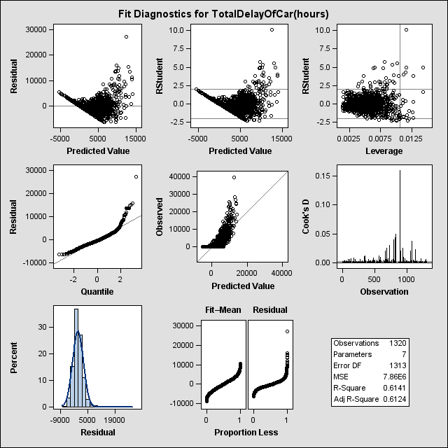
Figure 19. Chart. Fit diagnostics for total travel delay of light-duty vehicles.
In general, any systematic pattern in residuals indicates a violation in assumptions and systematic error (figure 19). In this model, it appears that the linearity assumption is violated because the residuals are not scattered randomly around zero and do not form a clear pattern. Also, the variance of residuals seems to have two values and that value is not constant.
It shows that accuracy of the model decreases as TDc increases. This problem is known as heteroscedasticity.

Figure 20. Chart. Plot of residuals for total travel delay of light-duty vehicles.

Figure 21. Chart. Plot of R-student residuals for total travel delay of light-duty vehicles.
Looking at the Quantile-Quantile plot (figure 21) the slope of the curve of the plotted points increases from left to right, which indicates that a theoretical distribution skewed to the right, such as a log-normal distribution, might better fit the data. In addition, the mild curve indicates a small shape parameter for the chosen distribution (i.e. σ for log-normal). Cook’s Distance (figure 23) shows outlier points, as all data points are not within a distance of two units of residual of the zero line. However, since the data result from designed experiments, we cannot eliminate the outliers with this method.

Figure 22. Chart. Quantile-Quantile plot for total travel delay of light-duty vehicles.

Figure 23. Chart. Outlier and leverage diagnostics for total travel delay of light-duty vehicles.
As part of additional analysis, the residuals are plotted separately for each explanatory variable (figure 22). Since the variables are uncorrelated by design, each graph shows the direct relationship of the dependent variable and the explanatory variable. Travel delays of light-duty vehicles seem to have a nonlinear relationship with a number of available lanes. The residuals suggest data-fitting functions, such as log-normal distributions. Incident duration has a random scatter plot suggesting a quadratic relationship between incident duration and travel delay of cars. Also, variance is not constant and there is fanning.
Residuals of volume show cosine or bimodal distribution. Form Residuals associated with the FFS, truck composition, and gradient are also randomly scattered around zero; therefore, the linear assumption seems reasonable.
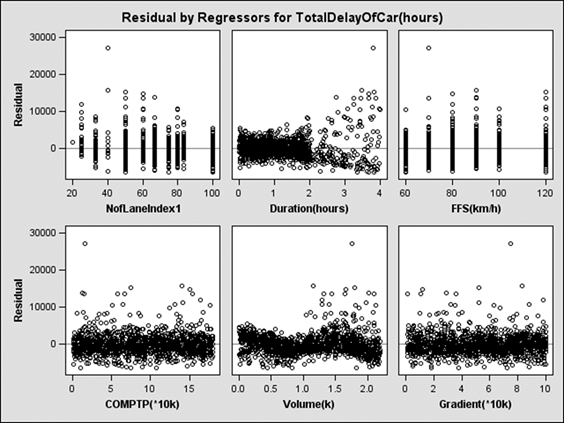
Figure 24. Chart. Scatterplots of residuals against explanatory variables.
Given these observations, to improve the model, new variables based on the above analysis were introduced to the model and the process was continued. These variables were developed from a variety of transformations involving the explanatory variables.
For travel delay of light-duty vehicles, residual graphs for the final fitted model were found, as seen in figure 25 and figure 26. Residuals are distributed normally around zero (figure 25) and systematic patterns of these models are eliminated (figure 26).

Figure 25. Chart. Normality of residuals for total delay of cars.

Figure 26. Chart. Standard residuals for total delay of cars.

