U.S. Department of Transportation
Federal Highway Administration
1200 New Jersey Avenue, SE
Washington, DC 20590
202-366-4000
Federal Highway Administration Research and Technology
Coordinating, Developing, and Delivering Highway Transportation Innovations
| SUMMARY REPORT |
| This summary report is an archived publication and may contain dated technical, contact, and link information |
|
| Publication Number: FHWA-HRT-18-037 Date: September 2017 |
Publication Number: FHWA-HRT-18-037 Date: September 2017 |
The experiment was conducted on seven rolling roadway segments in the States of Virginia and Maryland, with a total experimental mileage of around 47 miles. The types of terrain characterizing these segments vary from mildly rolling to very hilly.
Power analyses were conducted on initial testing data using GPower statistical software (Faul et al., 2007) to determine the required number of runs. Twenty runs of data were collected by running a preset speed profile on one of the experimental segments. Corresponding fuel consumption data were recorded. The analysis results show that four, three, and two samples are needed for segment lengths of 2, 6, and 10 miles, respectively. Therefore, based on the segment length, four runs of data were collected and averaged in our experiment to account for certain random factors. Additionally, experimental runs on the same segment were collected on the same day to avoid confounding factors such as temperature, wind speed, and pavement condition that vary from day to day.
Detailed roadway elevation profile data are not widely available for all roads. This study attempts to use the PinPoint device and PPP GPS service to collect elevation data. This method is preferred in the future, especially when all vehicles can be equipped with such advanced sensors. Note that this roadway profile information is usually collected through roadway survey and design documents from State DOT construction divisions, and are usually only available for newly constructed, major roads. However, given that roadway geometry data collected via connected vehicle technology are much more accessible than those from design/survey documents, it is believed that CV geometry data are more likely to be used as input for future eco-drive applications than survey data. Therefore, this experiment purposefully uses CV geometry data as inputs. It is one of the many design elements this experiment adopts to ensure the eco-drive application is tested under the most realistic environment.
In the experiment, two scenarios are tested:
Baseline: The benchmark is regular cruise control with cruising speeds set to corresponding roadway speed limits.
Eco-Drive: For eco-drive scenarios, vehicles will be given an optimal speed profile and will be controlled by the secondary speed controller in real time to follow the recommended speeds.
Fuel consumption was recorded, and the set of parameters that yield the lowest fuel consumption were selected (speed commands are given 13 meters (45 feet) in advance, geofence size/radius = 2 meters, maximum acceleration = 1 meter/sec,2 and speed command interval = 10 meters).
Detailed roadway elevation profile data are not widely available for all roads. This study attempts to use the PinPoint device and PPP GPS service to collect elevation data. This method is anticipated to be preferred in the future, especially when all vehicles can be equipped with such advanced sensors. Vehicle elevation data were compared with the ground truth elevation profile obtained from construction design and survey. The accuracy of the enhanced GPS data was then validated. The absolute value of elevation generally stays within a 3 percent error. Notably, this inaccuracy is mostly because of systematic errors, and the relative error reach is within 1 percent after a certain level of data smoothing. This confirms the validity of using such advanced GPS services for roadway profile data collection.
Experimental data were analyzed at the segment and subsegment level to derive insights into the effectiveness of eco-drive. The subsegment level analysis compared average fuel consumption of baseline and eco-drive runs at each of the seven sites. Understanding of general eco-drive performance was obtained through close examination of vehicle speed, acceleration, brake status, brake percentages, and instantaneous fuel consumption profiles. The segment-level analysis, however, does not reveal actual contributors to differences in fuel saving. Therefore, subsegment-level analysis was performed by applying linear models. Variables describing the subsegment characteristics were extracted, and a linear model was established to reveal the impacts of different characteristics on fuel saving potential.
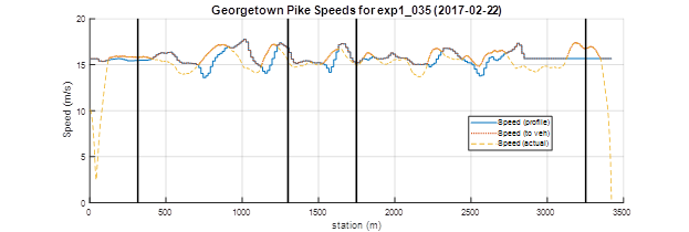
Figures 8(a) and (b) demonstrate actual speed data collected from two experimental runs (eco-drive and baseline) on Georgetown Pike as compared to commanded speed. The blue solid line shows the actual speed profile and the red dotted line shows the modified speed commands from the real-time secondary controller. The yellow dashed line is the actual speed profile when the vehicle tried to follow the speed commands (red dotted line). It can be seen from figure 8(a) that the vehicle can generally follow the speed commands closely even on this rolling terrain. At 1500 meters, the data between two black bars are removed from the fuel consumption calculation because there is a traffic light at which the vehicle stops during some runs. Figure 8(b) shows the baseline scenario in which speed commands were set to the speed limit of 35 mph (15.6 m/s). The actual speed profile (yellow dashed line) is compared with optimal speed commands. It shows that (adaptive) cruise control always tries to maintain the target speed, and thus it brakes frequently on downhill segments and applies the gas frequently on uphill segments. It is easy to predict that this behavior may result in extra fuel consumption. A closer look at the data in figure 8(a) reveals the smoothness of the vehicle trajectory, which is mostly because of a well-tuned PID control.

(b) Georgetown Pike example speed profile for baseline.
Figure 8. Speed Profile results at the segmental level for example runs (Source: FHWA).
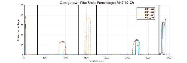
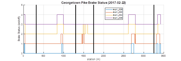
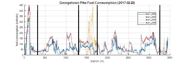
Figures 9(a) through (d) plot data from four experimental runs on vehicle acceleration, brake percentage, and brake status. Among these data, runs with labels of “exp1_029” and “exp1_030” are eco-drive runs, and those labeled “exp1_034” and “exp1_035” are baseline scenarios. The vehicle acceleration value and brake percentage of eco-drive runs are usually lower than the baseline runs. This is because the algorithm considers vehicle dynamics when generating the speed profile and the additional logic in the secondary real-time controller eliminates unnecessary braking relative to the baseline runs. The resulting fuel consumption benefits are reflected in figure 9(d). In many locations where acceleration was avoided, eco-drive runs consume much less fuel. Less braking and smaller brake percentages translate to a more effective transformation between potential and kinetic energy, thus less additional fuel is needed to provide the extra kinetic energy.

(b) Georgetown Pike brake percentage.

(c) Georgetown Pike brake status.

(d) Georgetown Pike fuel consumption for multiple runs.
Note: exp1_029 and exp1_030 are eco-drive runs, and exp1_034 and exp1_035 are baseline runs.
Figure 9. Experimental results at segmental level for example runs (Source: FHWA).
Table 1 details average results from each experimental site. Note that the travel times for the baseline and eco-drive scenarios are quite similar (mostly within a range of 5 percent) because the trajectory planning algorithm aims to maintain the same level of mobility while improving fuel consumption. The table also shows basic statistics as to instant fuel consumption throughout the experimental runs. As shown, the maximum instantaneous fuel consumption (mL/min) of the baseline runs is usually much larger than that of the eco-drive runs.
The total fuel consumption savings vary significantly, ranging from 2 percent to more than 20 percent. This result is expected because fuel use is highly dependent on attributes of the terrain, such as hill length and slope. The roadway profile of Georgetown Pike NB consists of constant, continuous uphill and downhill segments with steep grades (4–8 percent), and thus, logically, there is greater room for improvement. For roadway segments like GW Parkway NB, the savings are relatively small because the roadway vertical profile is mild and it includes a flat subsegment that generates very small fuel consumption differences between the baseline and eco-drive scenarios. Additional analysis at the subsegment level is needed to understand exactly what impacts fuel consumption benefits.
The algorithm speed commands are generated offline using a vehicle model and then fed to the vehicle longitudinal controller. To account for differences between the vehicle model and the actual vehicle (load, engine wear, transmission state, etc.) the actual vehicle speed was allowed to vary by 10 mph over or under the commanded speed. These differences, particularly the lack of direct control over transmission state, led to significant differences between the theoretical and measured fuel savings.
The subsegment-level analysis breaks down seven long segments listed in table 1 into many short subsegments, as illustrated in figure 10. The portion between two circles (one downhill and one uphill segment) is considered to be one subsegment. Fuel consumption savings were calculated as eco-drive fuel ÷ baseline fuel −1. In order to understand what attributes contribute the most to fuel consumption savings, the following subsegment characteristics were extracted for each subsegment: subsegment fuel consumption; uphill length (length of the uphill subsegment); uphill rise (elevation change of the uphill subsegment); uphill average slope (average slope along the uphill subsegment); downhill length (length of the downhill subsegment); downhill rise (elevation change of the downhill subsegment); downhill average slope (average slope along the downhill subsegment); and speed limit (distance-based average speed limit of the subsegment). To simplify the analysis, the uphill and downhill slopes were approximated using a straight line between the high point and low point. This slope is shown in the figure as black dotted lines.
Linear models were built to understand which roadway attributes contribute the most to fuel savings. Therefore, subsegment fuel consumption is the response variable, and others are used as predictors. In addition, attributes of the prior and following subsegments were also used as predictors. This is because the algorithm tends to consider the future rolling terrain profile and the remaining kinetic energy at the beginning of the current subsegment (or end of the prior subsegment). This is directly related to how much additional energy the vehicle needs to traverse the current subsegment.
Many of these predictors can be correlated; therefore, careful variable selection was conducted using a stepwise method and trial-and-error model construction (by removing highly correlated variables as measured by the Pearson correlation coefficient). The model with the best Akaike information criterion (AIC) value and prediction accuracy on test datasets was selected. Also, the final model presented below has been diagnosed and the response variable has been transformed using the box-cox method to ensure the assumptions of the linear models are satisfied.
Table 2 shows the results of the linear models. Note that interaction effects are considered in the original model, but those effects were neither significant nor selected in this final model. The R-squared value of the overall model is 0.705, indicating that 70 percent of the variance of fuel consumption saving variation can be captured by this model.
The fuel saving is calculated as eco-drive fuel ÷ baseline fuel −1, and therefore negative coefficients indicate more fuel saving. Uphill lengths of the current subsegment positively impact the fuel saving benefits, mostly because the secondary controller limits the acceleration value to 1 meter/sec2, and the baseline manufacturer (adaptive) cruise control usually uses large acceleration values on long hills to maintain cruising speed.
Subsegment waviness, as calculated using equation 24, is introduced to quantify the extent of waviness of a subsegment. Equation 25 adds waviness of all subsegments together to calculate overall waviness of a road segment, and table 1 shows these values for each experimental segment. The correlation between waviness and savings is generally minimal, except data for Georgetown Pike, where a large waviness value accompanies a large fuel savings. Otherwise, waviness cannot be directly correlated to fuel savings when the waviness values are similar, and this indicates that more complex relationship between the geometry and fuel savings may exist that are not captured in the linear model used in this paper to describe that relationship.
(24)

(25)
Where
wi = the waviness of subsegment i.
giu = average slope uphill.
gid = average slope downhill.
li = subsegment length.
W = overall segment waviness.
L = the overall length of the route.
Uphill length and average slope of the prior subsegment negatively impact savings. This result is expected because the large values of these two attributes mean that the vehicle can retain less kinetic energy when it climbs to the beginning of current subsegment. Meanwhile, the longer downhill length of the prior subsegment clearly results in larger benefits because the vehicle can accumulate more kinetic energy. Both the downhill and the uphill length of the next subsegment also significantly impact the actual saving of the current subsegment. It is difficult to obtain an intuitive explanation of the positive or negative impacts because, logically, the downstream subsegment should not impact upstream fuel consumption. This result, however, proves that the algorithm considers future rolling terrain when optimizing the speed profile, and it confirms the predictive nature of the algorithm.
The linear model can also be used to roughly estimate the benefits of eco-drive for any roadway segment. This is a useful tool for traffic management centers because they would only want to control vehicle speeds or provide recommended speed profiles for eco-drive on roadways where large benefits can be generated. Traffic management centers can initially use this model to identify all these potential roadway segments where eco-drive is desired, and the list of these segments can always be updated later when real fuel data are collected.
a (1), (0) and (2) indicates ego, prior, and next subsegments.
b Significance codes: 0: ‘***’; 0.001: ‘**’; 0.01: ‘*’; 0.05: ‘.’; 0.1; ‘ ’: 1.
The linear regression model is expressed in equation 26.

(26)
Where
βi = the coefficient estimate.
xi = the corresponding variable.
i ranges from 1 to the number of variables (in this case, i = {1, …, 10}).