U.S. Department of Transportation
Federal Highway Administration
1200 New Jersey Avenue, SE
Washington, DC 20590
202-366-4000
Federal Highway Administration Research and Technology
Coordinating, Developing, and Delivering Highway Transportation Innovations
| REPORT |
| This report is an archived publication and may contain dated technical, contact, and link information |
|
| Publication Number: FHWA-HRT-13-077 Date: January 2014 |
Publication Number: FHWA-HRT-13-077 Date: January 2014 |
CMFs used in the AASHTO HSM can be derived from the predictive models developed in chapter 4 of this current report. A CMF is a factor that represents the effect on crash frequency for a given crash severity level of varying geometric design or traffic control feature of interest (or a particular combination of geometric design or traffic control feature). Each CMF has a nominal value of 1.0 for a specified base condition. A CMF with a value greater than 1.0 represents a condition for which more crashes would be expected for the base condition. A CMF with a value less than 1.0 represents a condition for which fewer crashes would be expected than for the base condition. The base condition for all CMFs developed in this research is a level tangent roadway.
For each combination of alignment type (and for FI crashes and PDO crashes), CMFs were calculated as the ratio of the predicted crash frequency for a given horizontal curve and grade combination to the predicted crash frequency for the level tangent base condition. The following subsections provide equations for each CMF and figures illustrating the relationships of each roadway parameter to crash frequency and to the relevant CMF. Sample CMF calculations are also presented.
CMFs for horizontal curves and tangents on straight grades can be derived from figure 12 and figure 13 as follows shown in figure 39 and figure 40*:
*Modified on November 16, 2014

Figure 39. Equation. FI CMF for horizontal curves and tangents on straight grades.

Figure 40. Equation. PDO CMF for horizontal curves and tangents on straight grades.
The functional relationships shown in figure 12 (crashes/mi/year) and figure 39 (CMF) for FI crashes are illustrated in figure 41 for combinations of horizontal curve lengths and percent grades. Curve radius ranged from 100 to 11,460 ft; AADT was fixed at 2,000 vehicles/day; the median traffic volume was for rural two-lane roadways in the database; the horizontal curve length was set at 0.05, 0.10, 0.15, and 0.20 mi; and grade was set at level (i.e., 0 percent) and 1 to 6 percent in increments of 1 percent. Similarly, figure 42 illustrates the relationships shown in figure 13 and figure 40 for PDO crashes.
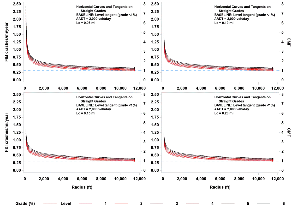
Figure 41. Graph. Predicted FI crashes/mi/year and CMFs for horizontal curves and tangents on straight grades.
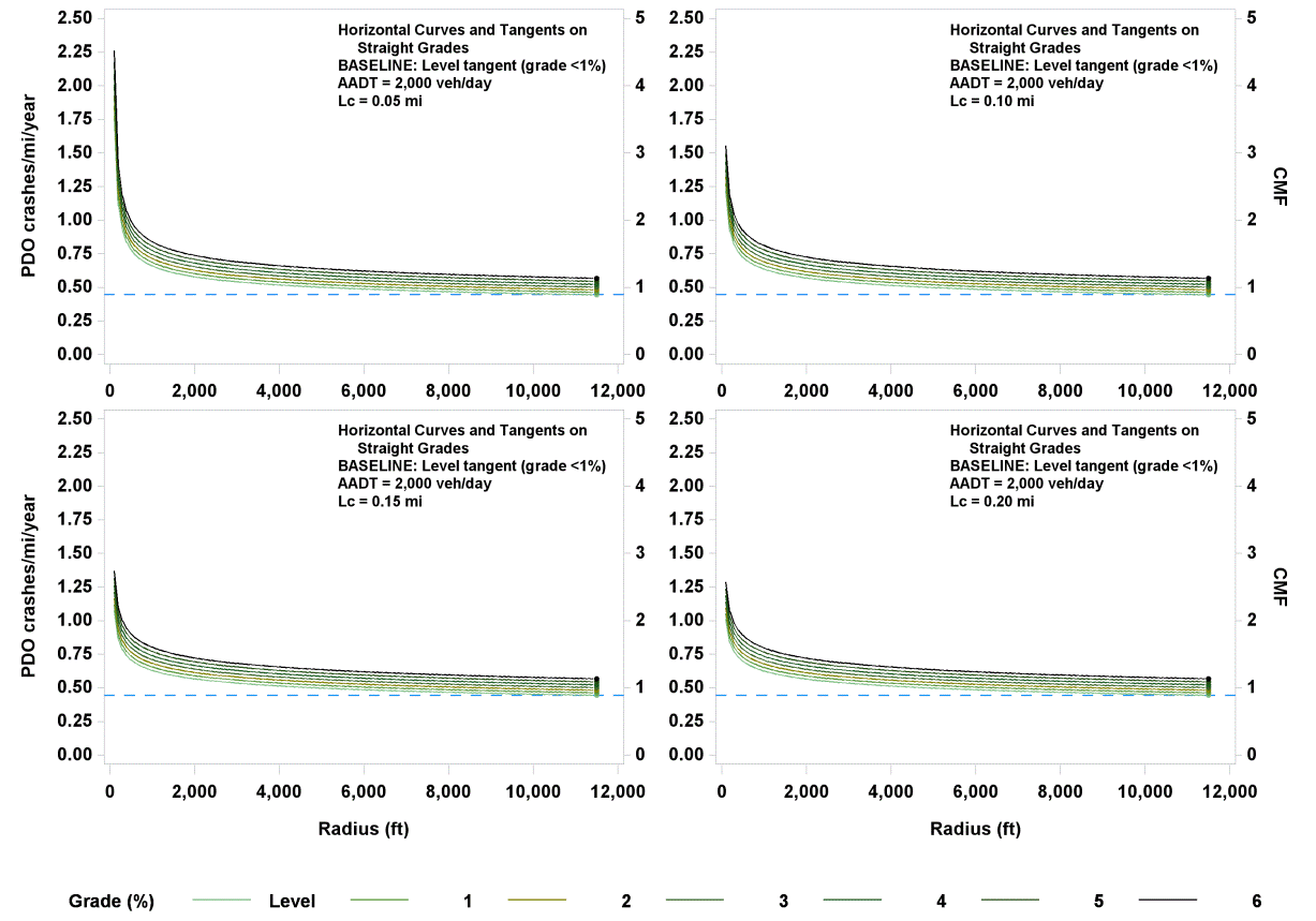
Figure 42. Graph. Predicted PDO crashes/mi/year and CMFs for horizontal curves and tangents on straight grades.
In figure 41 and figure 42, crashes/mi/year are shown on the left y-axis, and the corresponding CMFs are shown on the right y-axis. The dotted blue line corresponds to a base condition tangent with an AADT of 2,000 vehicles/day and therefore has a CMF of 1.0.
To calculate CMF for FI or PDO crashes for a given horizontal curve on a level or nonlevel grade or a tangent on a nonlevel grade, G (percent), R (ft), and LC (mi) are substituted in figure 39 or figure 40. Example CMFs were calculated for rural two-lane roadways with a R of 1,433 or 5,730 ft; LC of 0.05, 0.10, and 0.50 mi; and G ranging from level to 6 percent. The results are shown in table 17 for rural two-lane roadways with AADTs from 200 to 26,000 vehicles/day.
Table 17. Example CMFs for FI and PDO crashes on horizontal curves and tangents on straight grades.
Grade |
Tangent |
R = 1,433 ft |
R = 5,730 ft |
|||||||||
Horizontal Curve Length (mi) |
Horizontal Curve Length (mi) |
|||||||||||
0.05 |
0.10 |
0.50 |
0.05 |
0.10 |
0.50 |
|||||||
CMFs for FI Crashes |
||||||||||||
Level |
1.00 |
1.57 |
1.53 |
1.49 |
1.15 |
1.15 |
1.14 |
|||||
1 |
1.04 |
1.64 |
1.59 |
1.56 |
1.20 |
1.20 |
1.19 |
|||||
2 |
1.09 |
1.71 |
1.67 |
1.63 |
1.25 |
1.25 |
1.25 |
|||||
3 |
1.14 |
1.79 |
1.74 |
1.70 |
1.31 |
1.31 |
1.30 |
|||||
4 |
1.19 |
1.87 |
1.82 |
1.78 |
1.37 |
1.36 |
1.36 |
|||||
5 |
1.25 |
1.95 |
1.9 |
1.86 |
1.43 |
1.42 |
1.42 |
|||||
6 |
1.30 |
2.04 |
1.98 |
1.94 |
1.49 |
1.49 |
1.48 |
|||||
CMFs for PDO Crashes |
||||||||||||
Level |
1.00 |
1.38 |
1.35 |
1.32 |
1.10 |
1.10 |
1.10 |
|||||
1 |
1.04 |
1.44 |
1.40 |
1.38 |
1.15 |
1.14 |
1.14 |
|||||
2 |
1.08 |
1.49 |
1.46 |
1.43 |
1.20 |
1.19 |
1.19 |
|||||
3 |
1.13 |
1.56 |
1.52 |
1.49 |
1.25 |
1.24 |
1.24 |
|||||
4 |
1.17 |
1.62 |
1.58 |
1.55 |
1.30 |
1.29 |
1.29 |
|||||
5 |
1.22 |
1.69 |
1.65 |
1.62 |
1.35 |
1.35 |
1.34 |
|||||
6 |
1.27 |
1.76 |
1.72 |
1.69 |
1.41 |
1.40 |
1.40 |
|||||
In any given column in table 17, the CMFs show the increasing effect on crashes of an increasing grade for a horizontal curve or tangent on a straight grade. In any given row for a given curve radius, the CMFs show the increasing effect on crashes of horizontal curve length. The decreasing effect on crashes of longer curve radii is shown by comparing any two columns for the same curve length between the two radii. The effect of a short and sharp curve (due to the last term in figure 39 and figure 40) is reflected in the high CMFs in the third column of the table. As the curve radius increases and becomes a tangent for all practical purposes, the CMFs for the curve approach in value those of a tangent with the same percent grade. When percent grade nears zero (level roadway) and the radius becomes infinite (tangent roadway), the roadway becomes a level tangent, and CMF becomes 1.
CMFs for horizontal curves and tangents at type 1 crest vertical curves can be derived from figure 18 and figure 19 as follows shown in figure 43 and figure 44 *:
*Modified on November 16, 2014

Figure 43. Equation. FI CMF for horizontal curves and tangents at type 1 crest vertical curves.

Figure 44. Equation. PDO CMF for horizontal curves and tangents at type 1 crest vertical curves.
The functional relationships shown in figure 18 (crashes/mi/year) and figure 43 (CMF) for FI crashes are illustrated in figure 45 for selected values of K. Curve radius ranged from 100 to 11,460 ft, AADT was fixed at 2,000 vehicles/day, and LVC was fixed at 500 ft, the median LVC in the database. Values of K were set at 250, 125, 83, 63, and 50, which correspond to a grade difference of 2, 4, 6, 8, and 10 percent, respectively, for a curve length of 500 ft. Similarly, figure 46 illustrates the relationships shown in figure 19 and figure 44 for PDO crashes.
To calculate CMF for FI or PDO crashes for a given horizontal curve at a type 1 crest vertical curve, the actual values of R (ft), LVC (ft), and parameter K (ft/percent) are substituted in figure 43 or figure 44. Example CMFs were calculated for rural two-lane roadways with an LVC of 500 ft, R of 1,433 or 5,730 ft, and K values of 250, 125, 83, 63, and 50 ft/percent using figure 43 and figure 44. The results are shown in table 18 for rural two-lane roadways with AADTs from 200 to 26,000 vehicles/day and LVC of 500 ft.
Table 18. Example CMFs for FI and PDO crashes on horizontal curves and tangents at type 1 crest vertical curves.
K |
Tangent |
FI CMFs |
PDO CMFs |
||
R = 1,433 ft |
R = 5,730 ft |
R = 1,433 ft |
R = 5,730 ft |
||
250 |
1.0 |
1.07 |
1.02 |
1.04 |
1.01 |
125 |
1.0 |
1.15 |
1.04 |
1.08 |
1.02 |
83 |
1.0 |
1.24 |
1.05 |
1.12 |
1.03 |
63 |
1.0 |
1.33 |
1.07 |
1.16 |
1.04 |
50 |
1.0 |
1.42 |
1.09 |
1.20 |
1.05 |
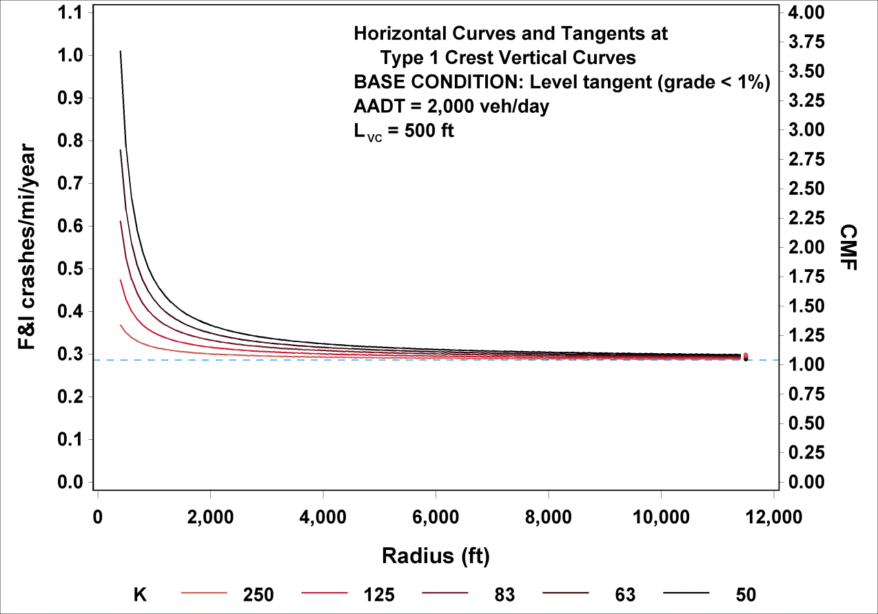
Figure 45. Graph. Predicted FI crashes/mi/year and CMFs for horizontal curves and tangents at type 1 crest vertical curves.
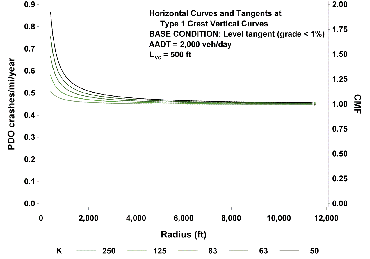
Figure 46. Graph. Predicted PDO crashes/mi/year and CMFs for horizontal curves and tangents at type 1 crest vertical curves.
In any given column in table 18, the CMFs show the increasing effect on crashes of a decreasing K (steeper crest) of a horizontal curve at a type 1 crest vertical curve. This effect is less pronounced for PDO crashes than for FI crashes. The combined effect of a sharp horizontal curve on a steep vertical crest is reflected in the last rows of the third and fifth columns. When K becomes infinite (i.e., level roadway) and R becomes infinite (i.e., tangent roadway), the roadway becomes a level tangent, and CMF becomes 1.0.
CMFs for horizontal curves and tangents at type 1 sag vertical curves can be derived from
figure 25 and figure 26 as follows shown in figure 47 and figure 48*:
*Modified on November 16, 2014

Figure 47. Equation. FI CMF for horizontal curves and tangents at type 1 sag vertical curves.

Figure 48. Equation. PDO CMF for horizontal curves and tangents at type 1 sag vertical curves.
The functional relationships shown in figure 25 (crashes/mi/year) and figure 47 (CMF) for FI crashes are illustrated in figure 49 for K values of 250, 125, 83, 63, and 50. R ranged from 100 to 11,460 ft, AADT was fixed at 2,000 vehicles/day, and LVC was fixed at 500 ft. Similarly, figure 50 illustrates the relationships shown in figure 26 and figure 48 for PDO crashes.
To calculate CMF for FI or PDO crashes for a given horizontal curve at a type 1 sag vertical curve, the actual values of R (ft), LVC (ft), and parameter K (ft/percent) are substituted in figure 47 or figure 48. Example CMFs were calculated for rural two-lane roadways with a vertical curve length of 500 ft, an R of 1,433 or 5,730 ft, and K values of 250, 125, 83, 63, and 50 using figure 47 and figure 48. The results are shown in table 19 for rural two-lane roadways with AADTs from 200 to 26,000 vehicles/day.
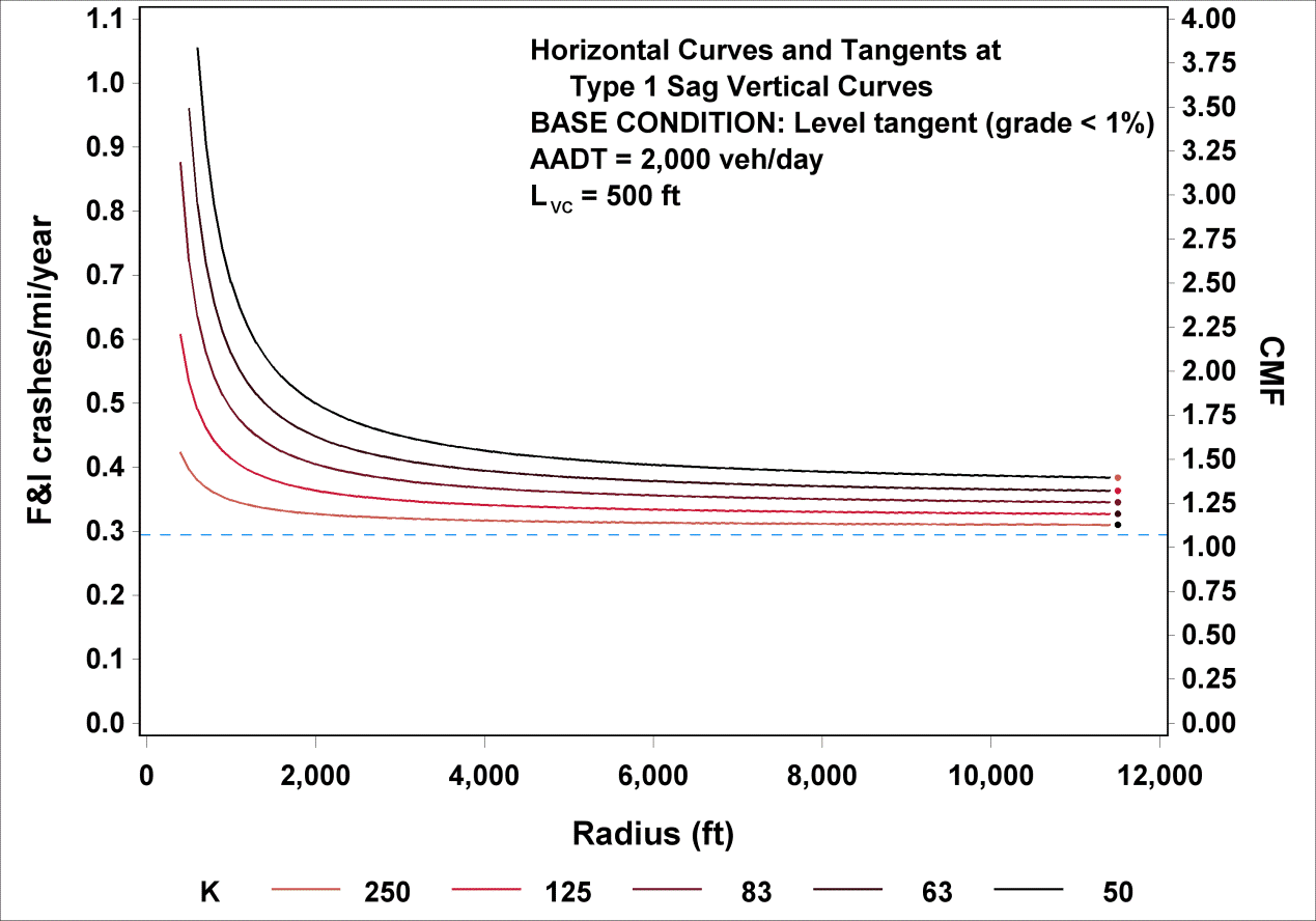
Figure 49. Graph. Predicted FI crashes/mi/year and CMFs for horizontal curves and tangents at type 1 sag vertical curves.
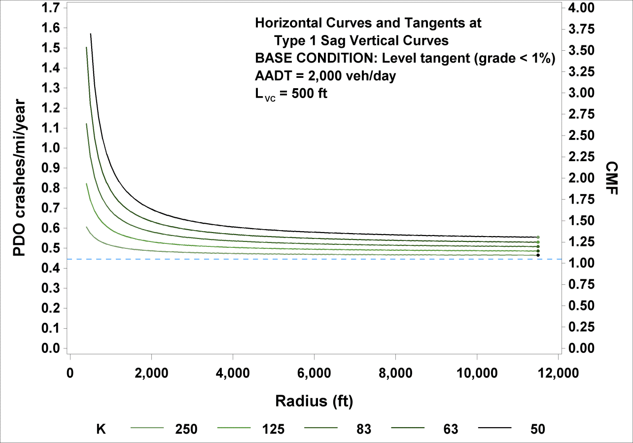
Figure 50. Graph. Predicted PDO crashes/mi/year and CMFs for horizontal curves and tangents at type 1 sag vertical curves.
Table 19. Example CMFs for FI and PDO crashes on horizontal curves and tangents at type 1 sag vertical curves.
K |
FI CMFs |
PDO CMFs |
||||
Tangent at Sag |
R = 1,433 ft |
R = 5,730 ft |
Tangent at Sag |
R = 1,433 ft |
R = 5,730 ft |
|
250 |
1.04 |
1.14 |
1.07 |
1.04 |
1.12 |
1.05 |
125 |
1.09 |
1.30 |
1.14 |
1.07 |
1.25 |
1.11 |
83 |
1.13 |
1.49 |
1.21 |
1.11 |
1.39 |
1.17 |
63 |
1.18 |
1.68 |
1.29 |
1.15 |
1.55 |
1.24 |
50 |
1.23 |
1.93 |
1.38 |
1.19 |
1.74 |
1.31 |
In any given column in table 19, CMFs show the increasing effect on crashes of decreasing K (sharper sag) for a horizontal curve or tangent at a type 1 sag vertical curve. This effect is slightly less pronounced for PDO than for FI crashes. When K becomes very large (i.e., level roadway), and R becomes infinite (i.e., tangent roadway), the roadway becomes a level tangent, and CMF becomes 1.0.
CMFs for horizontal curves and tangents at type 2 crest vertical curves can be derived from figure 32 and figure 33 as follows shown in figure 51 and figure 52*:
*Modified on November 16, 2014

Figure 51. Equation. FI CMF for horizontal curves and tangents at type 2 crest vertical curves.

Figure 52. Equation. PDO CMF for horizontal curves and tangents at type 2 crest vertical curves.
The functional relationships shown in figure 32 (crashes/mi/year) and figure 51 (CMF) for FI crashes are illustrated in figure 53 for an R range from 100 to 11,460 ft and AADTs of 1,000, 2,000, 4,000, and 7,000 vehicles/day (corresponding approximately to the 25th, 50th, 75th, and 90th percentile AADTs for rural two-lane highways in the database). Similarly, figure 54 illustrates the relationships shown in figure 33 and figure 52 for PDO crashes.
To calculate CMF for FI or PDO crashes for a given horizontal curve at a type 2 crest vertical curve, the actual value of R (ft) is substituted in figure 51 or figure 52. Example CMFs were calculated for rural two-lane roadways with an R of 1,433, 5,730, or 11,460 ft using figure 51 and figure 52. The results are shown in table 20 for rural two-lane roadways with AADTs from 200 to 26,000 vehicles/day.
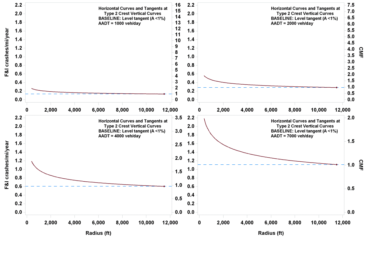
Figure 53. Graph. Predicted FI crashes/mi/year and CMFs for horizontal curves and tangents at type 2 crest vertical curves.
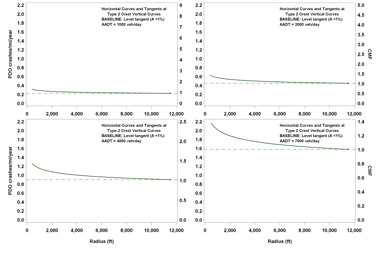
Figure 54. Graph. Predicted PDO crashes/mi/year and CMFs for horizontal curves and tangents at type 2 crest vertical curves.
Table 20. Example CMFs for FI and PDO crashes on horizontal curves and tangents at type 2 crest vertical curves.
FI CMFs |
PDO CMFs |
||||
R = 1,433 ft |
R = 5,730 ft |
R = 11,460 ft |
R = 1,433 ft |
R = 5,730 ft |
R = 11,460 ft |
1.52 |
1.15 |
1.00 |
1.23 |
1.07 |
1.00 |
Only R of the horizontal curve at a type 2 vertical crest has an effect on crash rates, with increasing radii producing smaller CMFs. The effect of R is more pronounced for FI crashes than for PDO crashes. When R becomes infinite, the roadway becomes a tangent, and CMF becomes 1.0 regardless of the vertical curve characteristics.
Because this CMF lacks any measure of vertical alignment, consideration may be given to replacing this CMF with a CMF based on figure 10 and figure 11.
CMFs for horizontal curves and tangents at type 2 sag vertical curves can be derived from
figure 37 and figure 38 as follows shown in figure 55 and figure 56*:
*Modified on November 16, 2014

Figure 55. Equation. FI CMF for horizontal curves and tangents at type 2 sag vertical curves.

Figure 56. Equation. PDO CMF for horizontal curves and tangents at type 2 sag vertical curves.
The functional relationships shown in figure 37 (crashes/mi/year) and figure 55 (CMF) for FI crashes are illustrated in figure 57 for an R range from 100 to 11,460 ft and AADTs of 1,000, 2,000, 4,000, and 7,000 vehicles/day. Similarly, figure 58 illustrates the relationships shown in figure 38 and figure 56 for PDO crashes for K values of 250, 125, 83, 63, and 50; curve radii ranging from 100 to 11,460 ft; and AADT fixed at 2,000 vehicles/day.
To calculate CMF for FI crashes for a given horizontal curve at a type 2 sag vertical curve, the actual value of R (ft) is substituted in figure 55. To calculate CMF for PDO crashes, the actual value of R (ft), LVC, and K are substituted in figure 56. Example FI CMFs were calculated for rural two-lane roadways with an R of 1,433, 5,730, or 11,460 ft using figure 55. Example PDO CMFs were calculated using figure 56 for rural two-lane roadways with an R of 1,433 or 5,730 ft, an LVC of 500 ft, and A values ranging from 2 to 10 percent. The results are shown in table 21 for FI crashes and table 22 for PDO crashes for rural two-lane roadways with AADTs from 200 to 26,000 vehicles/day.
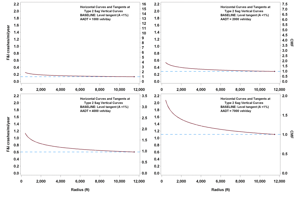
Figure 57. Graph. Predicted FI crashes/mi/year and CMFs for horizontal curves and tangents at type 2 sag vertical curves.
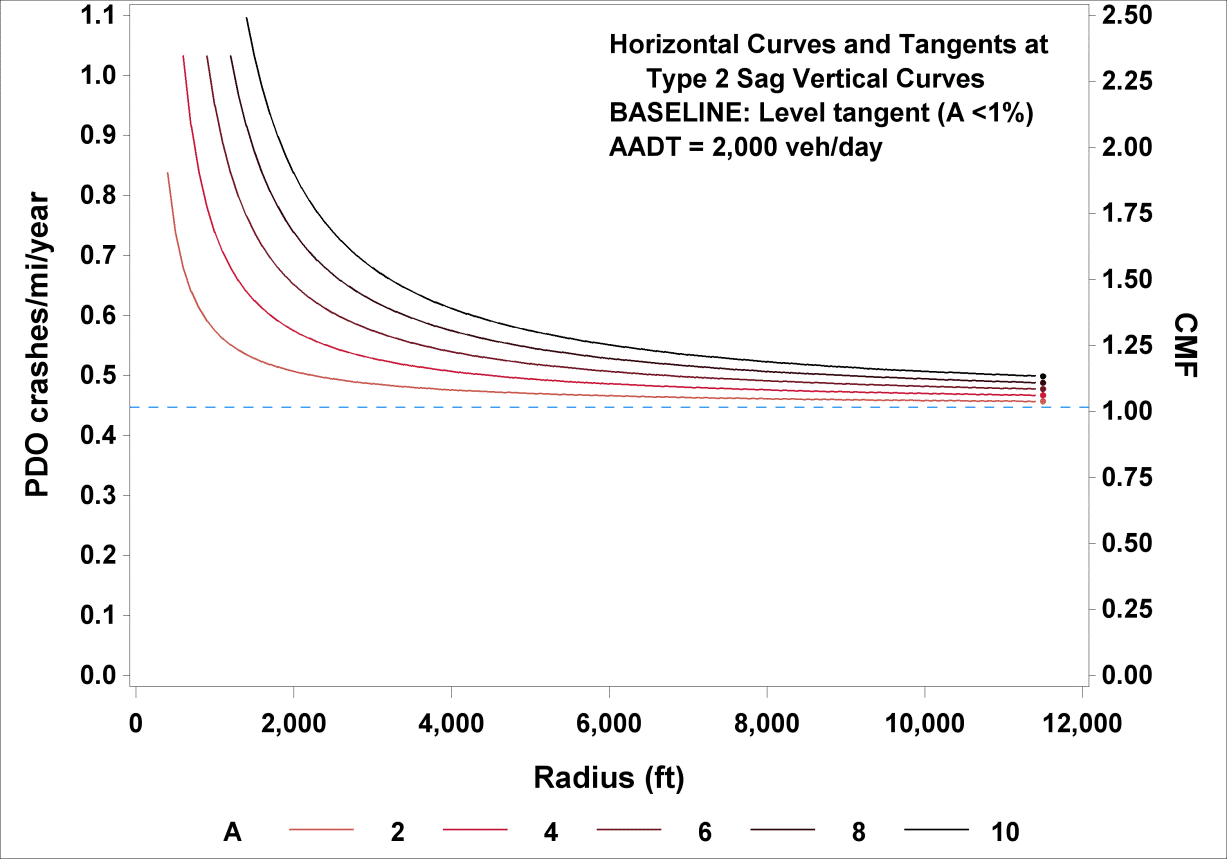
Figure 58. Graph. Predicted PDO crashes/mi/year and CMFs for horizontal curves and tangents at type 2 sag vertical curves.
Table 21. Example CMFs for FI crashes on horizontal curves and tangents at type 2 sag vertical curves.
FI CMFs |
||
R = 1,433 ft |
R = 5,730 ft |
R = 11,460 ft |
1.48 |
1.14 |
1.00 |
Table 22. Example CMFs PDO crashes on horizontal curves and tangents at type 2 sag vertical curves.
A |
PDO CMFs |
||
R = 1,433 ft |
R = 5,730 ft |
R = 11,460 ft |
|
All tangents |
1.00 |
1.00 |
1.00 |
2 |
1.19 |
1.04 |
1.02 |
4 |
1.42 |
1.09 |
1.04 |
6 |
1.69 |
1.14 |
1.07 |
8 |
2.02 |
1.19 |
1.09 |
10 |
2.40 |
1.24 |
1.12 |
Only R of the horizontal curve at a type 2 vertical sag has an effect on FI crash rates, with increasing radii producing smaller CMFs (see table 21). When R becomes infinite, the roadway becomes a tangent and CMF becomes 1.0 regardless of the characteristics of the vertical curve. Only the interaction term of A and inverse R has an effect on PDO crash rates (see table 22), highlighting the joint effect of sharp horizontal curves at steep vertical curves on PDO crashes. When the initial and final grade difference, A, nears zero (i.e., level roadway) and the R becomes infinite (i.e., tangent roadway), the roadway becomes a level tangent, and CMF becomes 1.0.
Because this CMF (at least for FI crashes) lacks any measure of vertical alignment, consideration may be given to replacing this CMF with a CMF based on figure 10 and figure 11.
This study provides separate CMFs for FI and PDO crashes. At some future time, the AASHTO HSM may be structured to provide separate CMFs by severity level for all CMFs. In the meantime, if users want a CMF for total crashes (i.e., all crash severity levels combined), it can be computed from the results in this report as follows shown in figure 59*:
*Modified on November 16, 2014

Figure 59. Equation. CMF for combined crash severity level.
Where:Values used for PFI and PPDO must always sum to 1.0. Values of PFI and PPDO indicated for rural two-lane highways in AASHTO HSM table 10-3 (PFI = 0.321 and PPDO = 0.679) may be used, or users may develop values for PFI and PPDO from their agencies’ data.(1)
The current AASHTO HSM presents separate CMFs for horizontal curves and straight grades, as seen as CMFHC in figure 3 and CMFG in figure 5, respectively.(1) The combined effect of horizontal curves and grades is represented in the AASHTO HSM as the product of CMFHC and CMFG. Figure 60 illustrates a comparison of CMFs for horizontal curves on straight grades developed in this study, and shown in figure 39 and figure 40 for FI and PDO crashes, respectively, to the combined AASHTO HSM CMF, holding length of horizontal curve and radius constant while varying percent grade. Figure 61 is an analogous plot, keeping the length of horizontal curve and percent grade constant while varying the radius of horizontal curve.
The plots show that the new CMF for FI crashes is consistently larger than the new CMF for PDO crashes. This represents an advance in knowledge over the AASHTO HSM, which treats CMFs for all severity levels as equal.(1) The plots also show that the new CMFs are generally larger than the combined AASHTO HSM CMFs, except that the new CMF for PDO crashes is smaller than the existing CMFs for horizontal curves with short radii. No other comparisons between the HSM CMFs and the CMFs developed in this study are relevant because the AASHTO HSM does not address the safety effects of crest or sag vertical curves.
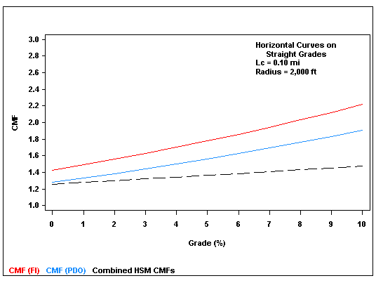
Figure 60. Graph. Comparison of CMFs developed in this study to the combined AASHTO HSM CMFs for horizontal curves and grades for fixed radius and varying percent grades.(1)
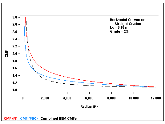
Figure 61. Graph. Comparison of CMFs developed in this study to the combined AASHTO HSM CMFs for horizontal curves and grades for fixed percent grade and varying radii.(1)