Active Traffic Management: Comprehension, Legibility, Distance, and Motorist Behavior in Response to Selected Variable Speed Limit and Lane Control Signing

Chapter 5. Driver DecisionMaking under Visual Clutter

This second simulation study used the same scenarios as the previous simulation study. The gantries for the per-lane ATM signs contained guide signs, but no side-mounted CMSs with supplemental roadway messages. The arrangement of the signs in this study was similar to the arrangement in the Minnesota deployment. In addition, two different levels of roadway clutter (low and moderate) were included on the sides of the road. The focus of this study was driver behavior and decisionmaking under different scenarios and varying levels of clutter.

Methods

The Simulator

The experiment was conducted using the FHWA Highway Driving Simulator. In the previous simulator experiment described in this report, the simulator's out-of-vehicle display consisted of a horizontal projection of 240 degrees onto a cylindrical screen. However, at the time of this study, the projectors had exceeded their life expectancy and were no longer capable of achieving the necessary brightness or resolution to support a sign study. Because the projectors could not be replaced within the timeframe of this study, three high-resolution LCD monitors were used to display the forward 104 degrees of the field-of-view. Two of the original projectors were used to complete the side portions of the 240 degrees horizontal display. The LCD monitors were mounted in the windshield area of the late model compact sedan as shown in figure 77.

Figure 77. Photo. The FHWA Highway Driving Simulator with LCD monitors.

Each of the LCD displays was 30 inches (76 cm) on the diagonal with a 16:10 aspect ratio. The LCD monitor resolutions were 2,560 horizontal pixels by 1,600 vertical pixels. LCD brightness was approximately 108 fl (370 cd/m²) with a typical contrast ratio of 1,000:1. The distance of the monitors from the driver's eye point varied with driver height and seat position. The nominal distance of the center monitor was 36 inches (91 cm). The right and left monitors were 39 and 49inches (99 and 124 cm), respectively, from the design eye point. All distance measurements were to the center of the respective displays. Images on each display were scaled to present a 1:1 correspondence with the real-world equivalents of the virtual world. All displays refreshed at 60 Hz. The minimum pixel response time on the LCD displays was 8 ms.

Rearview mirrors were simulated using 7.8- by 4.8-inch ((20 by 12-cm) color LCDs with 800pixels horizontally and 480 pixels vertically. These displays had a contrast ratio of 400:1. Left and right outside simulated mirrors were mounted over the sedan's original outside mirrors. The center-mounted rearview LCD was placed as near as possible to the location of the vehicle's original mirror.

The simulator's motion base was not enabled in this experiment. The car's instrument panel, steering, brake, and accelerator pedal all functioned in a manner similar to real-world compact cars.

The simulated vehicle was equipped with a hidden intercom system that enabled communications between the participant and a researcher who ran the experiment from a control room. The researcher in the control room could also view the face video from the eye-tracking system and thereby monitor the participant's well-being.

ATM Signs

The ATM signs used in this experiment were those shown in figure 43 through figure 49. These signs represented a selection of signs that were being used in ATM test deployments in Washington and Minnesota at the time of this study. Selection of these signs was based on the result of sign comprehension and preference testing done in a laboratory setting (see chapter 2). The sign gantries and mounting of the per-lane ATM signs were similar to that employed in the Minnesota field deployment.

Simulation Scenarios

The participants drove on a simulated eight-lane highway approximately 23 mi (37 km) in length. A 1-mi (1.61-km) section of freeway without overhead signs preceded the first overhead ATM sign. The ATM signs (gantries) were spaced every 0.5 mi (0.8 km) along the roadway. Because of limitations in the resolution of the simulator's projectors, all signs in the simulator were oversized so that their legibility distance approximated real-world legibility distances. In this experiment, signs were 1.25 times the size of their real-world equivalents. Figure 78 shows an example of an ATM sign at the start of an area in scenario 5 (speed reduction).

Figure 78. Screen capture. Example ATM signs for a speed reduction zone.

Each drive was composed of the following scenarios:

1. Resting condition for the signs (normal operations for all lanes).
2. Stalled vehicle closing 1 lane (right-center lane—lane 3).
3. Vehicle crash closing two left lanes (lanes 1 and 2).
4. Vehicle crash closing two right lanes (lanes 3 and 4 with exit ramp open).
5. Message in the event of slow-moving traffic in all lanes (speed reduction).

The traffic in this simulation was generated in the same manner as for the previous simulation experiment (see chapter 4).

Eye-Tracking System

The eye-tracking system and its setup was the same as for the previous simulation experiment (see chapter 4).

To quantify when and for how long participants looked at each ATM sign, a researcher used analysis software to indicate a ROI on individual frames of the recorded video image. An example of an ROI is shown in figure 78 (the halo around the signs). ROIs were created between the point a sign began to pass out of the driver's view and 10 s upstream of that point. Only one ROI for this experiment was created, which encompassed the four per-lane CMSs as well as the overhead guide signs.

Participants

Fifty-three participants successfully completed the simulation. However, only 43 participants (22 males and 21 females) produced usable eye-tracking data. Of these 43 participants, the mean age for males was 39 years old (range 18 to 73 years old) and the mean age for females was 44years old (range 18 to 76 years old).

Participants experienced low or medium levels of clutter depending on the clutter level. Of the participants who had usable eye-tracking data, 19 participants experienced the low clutter simulation, and 24 participants experienced the medium clutter simulation.

Results

In all figures, error bars indicate 95-percent confidence limits. Also, for ease of understanding, the scenarios have been coded in the figures as the following. There are two codes for scenario 5 (speed reduction) because participants viewed this scenario twice.

1. REST: Resting condition for the signs (normal operations for all lanes).
   
   
2. SVRCX: Stalled vehicle closing 1 lane (right-center lane - lane 3).
   
   
3. 2LFTX: Vehicle crash closing two left lanes (lanes 1 and 2).
   
   
4. 2RTXE: Vehicle crash closing two right lanes (lanes 3 and 4 with exit ramp open).
   
   
5. SLOW1/SLOW2: Message in the event of slow-moving traffic in all lanes (reduced speed).

Clutter Effect

First, all participants were included to analyze whether the level of clutter altered a driver's ability to successfully exit at the end of the drive (see table 29). Of these participants, 24 experienced the low clutter level and 29 experienced the medium clutter level. Chi-squared test results indicated there was no significant difference in exit-taking behavior for the two groups.

Table 29. Distribution (row percentages) for exit-taking behavior by clutter level for all participants (N = 53).

Next, only the 43 participants who produced usable eye-tracking data were included in a similar analysis of the effect of clutter (see table 30). Chi-squared test results indicated there was no significant difference in exit-taking behavior for the two groups.

Table 30. Distribution (row percentages) for exit-taking behavior by clutter level for all participants with usable eye-tracking data (N = 43).

Lane Choice and Speed Behavior

During data collection, researchers observed a participant's lane position following each gantry in the scenario. In scenario 1 (resting condition), three observations were recorded, one for each gantry. This scenario was presented to each participant at the beginning of the drive and then in between each of the other scenarios. Table 31 shows the distribution (row percentages) of lane choice across participants for each recorded observation. Chi-squared test results indicated there was no significant association between the observation in the scenario and lane choice. Overall, participants tended to stay in lane 3 as initially instructed by the researcher.

Table 31. Distribution (row percentages) of lane choice by DCZ for scenario 1 (resting condition).

— Indicates 0 percent.

In scenario 2 (stalled vehicle), six observations were recorded, one for each of the gantries. Table 32 shows the distribution (row percentages) of lane choice for each recorded observation. Chi-squared test results indicated there was a significant association between the observation in the scenario and lane choice (χ² (10) = 130.82, p < 0.001). The data suggest that the participants exited lane 3 in accordance with the instructions on the ATM signs. Once the stalled vehicle was encountered (between the fifth and sixth gantries), participants reentered lane 3.

Table 32. Distribution (row percentages) of lane choice by DCZ for scenario 2 (stalled vehicle).

— Indicates 0 percent.

Figure 79 shows the speed profile for this scenario. Unlike the previous experiment (see chapter4), VSL signs were used in this experiment to slow the traffic down as it approached the stalled vehicle. Also, in contrast to the previous experiment, participants were not presented supplemental roadway information messages on a side-mounted CMS in this experiment. The speed profile shows that the participants initially decreased their speeds in response to the VSL signs but then sped up throughout the scenario as they approached the stalled vehicle. By the time the stalled vehicle was encountered, the participants were driving about 10 mi/h (16 km/h) slower than the facility posted speed limit (65 mi/h (105 km/h)) but significantly faster than the posted speed limits shown on the last VSL sign (shown on gantry 2).

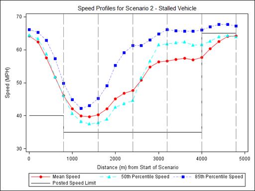
1 mi/h = 1.61 km/h.
1 ft = 0.305 m.

Figure 79. Graph. Speed profile for scenario 2 (stalled vehicle).

In scenario 3 (two left lanes closed), six observations were recorded, one for each of the gantries. Table 33 shows the distribution (row percentages) of lane choice for each recorded observation. Chi-squared test results indicated there was no significant association between the observation in the scenario and lane choice. The data suggest that participants exited the two left lanes (lanes 1 and 2) in accordance with the instructions on the ATM signs.

Table 33. Distribution (row percentages) of lane choices by DCZ for scenario 3 (two left lanes closed).

— Indicates 0 percent.

Figure 80 shows the speed profile for this scenario. VSL signs were used in this experiment to slow the traffic down as it approached the lane closure. Participants initially decreased their speeds in response to the VSL signs but then increased their speeds throughout the scenario. By the time they reached the crashed vehicles, participants were on average traveling about 10 mi/h (16 km/h) slower than the facility posted speed limit (65 mi/h (105 km/h)) but faster than the posted speed limits shown on the last VSL sign (shown on gantry 2).

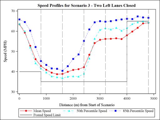
1 mi/h (MPH) = 1.61 km/h.
1 ft = 0.305 m.

Figure 80. Graph. Speed profile for scenario 3 (two left lanes closed).

In scenario 4 (two right lanes blocked, take exit), four observations were recorded, one for each of the four gantries. Table 34 shows the distribution (row percentages) of lane choice for each recorded observation. Chi-squared test results indicated there was a significant association between the observation in the scenario and lane choice (χ² (4) = 89.63, p < 0.001).

Table 34. Distribution (row percentages) of lane choices by DCZ for scenario 4 (two right lanes blocked, take exit; empty cells indicate 0 percent).

— Indicates 0 percent.

Figure 81 shows the speed profile for this scenario. VSL signs were used in this experiment to slow the traffic down as it approached the lane closure. Participants responded to the VSL signs by lowering their speeds. By the time the participants reached the exit, they were, on average, traveling about 10 mi/h (16 km/h) faster than the posted speed limit on the last VSL sign (shown on gantry 2) and 20 mi/h (32 km/h) slower than the facility posted speed limit (65 mi/h (105km/h)).

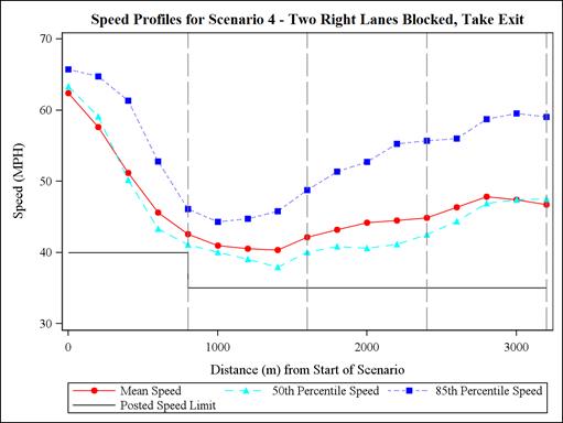
1 mi/h (MPH) = 1.61 km/h.
0.3 m = 1 ft = 0.305 m.

Figure 81. Graph. Speed profile for scenario 4 (two right lanes blocked, take exit).

Scenario 5 (speed reduction) was viewed twice by each participant (scenarios 5a and 5b, respectively). In scenario 5a (first speed reduction), six observations were recorded, one for each of the gantries. Table 35 shows the distribution (row percentages) of lane choice across participants for each recorded observation. Chi-squared test results indicated that there was no significant association between the observation in the scenario and lane choice. Overall, participants tended to stay in lane 3 as initially instructed by the researcher. Figure 82 shows the speed profile for this scenario. On average, the participants complied with the VSL signs.

Table 35. Distribution (row percentages) of lane choices by DCZ for scenario 5a (first speed reduction).

— Indicates 0 percent.

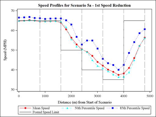
1 mi/h = 1.61 km/h.
1 ft = .305 m.

Figure 82. Graph. Speed profile for scenario 5a (first speed reduction).

In scenario 5b (second speed reduction), six observations were recorded, one for each of the gantries. Table 36 shows the distribution (row percentages) of lane choice across participants for each recorded observation. Chi-squared test results indicated that there was no significant association between the observation in the scenario and lane choice. Overall, participants tended to stay in lane 3 as initially instructed by the researcher. As with the first viewing, there was also high compliance with the VSL signs in this viewing of the scenario, and therefore the speed profile not shown.

Table 36. Distribution (row percentages) of lane choices by DCZ for scenario 5b (second speed reduction).

— Indicates 0 percent.

Glance Behavior

A glance toward an ROI was defined as when a participant registered 12 or more hits toward the ROI during a DCZ. If a glance occurred, then the number of hits was multiplied by 120 (the advertised sampling rate of the eye-tracking system) to calculate the duration.

Glance Probability

The overall probability of glancing, regardless of scenario, was 0.98. Thus, only descriptive statistics are reported in table 37.

Table 37. Probability of glancing by scenario.

Glance Duration

GEEs with a Gamma response distribution and identity link function were used to analyze the duration of a glance, given that a glance had occurred. In other words, no durations of 0 s were included in the analysis.

Results indicated that there was a statistically significant difference in the duration of a glance among the scenarios (χ² (4) = 100.65, p < 0.001). As is shown in figure 83, scenario 4 (two right lanes blocked, take exit) yielded the longest glance duration, and scenario 5b (second speed reduction) yielded the shortest glance duration.

Figure 83. Graph. Predicted mean glance duration by scenario.

Look Behavior

A look was defined as any accumulation of 7 or more hits on an ROI within a series of 12 frames (100 ms). A look began when this criterion was first met and terminated when the number of hits within the preceding 12 frames dropped below 7.

Look Probability

The overall probability of looking, regardless of scenario, was 0.98. Thus, only descriptive statistics are reported in table 38.

Table 38. Probability of looking by scenario.

Number of Looks

Repeated measures Poisson regression was used to determine whether the number of looks (assuming at least one look occurred) varied among the different scenarios. Results indicated there was a statistically significant difference in the number of looks across the scenarios (χ² (4) = 37.72, p < 0.001). As is shown in figure 84, scenario 4 (two right lanes blocked, take exit) resulted in the greatest number of looks, and scenario 5a (first speed reduction) yielded the smallest number of looks.

Figure 84. Graph. Predicted number of looks by scenario.

Look Duration

GEEs with a Gamma response distribution and identity link function were used to determine whether the duration of looks (assuming at least one look occurred) varied among the different scenarios. Results indicated there was a statistically significant difference in the number of looks across the scenarios (χ² (4) = 26.31, p < 0.001). As is shown in figure 85, scenario 4 (two right lanes blocked, take exit) resulted in the longest look duration, and scenario 5b (second speed reduction) yielded the shortest look duration.

Figure 85. Graph. Predicted mean look duration by scenario.

Fixation Behavior

A fixation was defined as seven consecutive gaze positions (60 ms) within a fixation radius of 4percent of the vertical image height (i.e., 15 pixels on the 372-pixel image) and centered on the first of the seven gaze positions that designated the start of a fixation. The fixation continued until there were six consecutive hits (50 ms) outside the fixation radius. For a simulated object 500 ft (152.4 m) ahead, the fixation radius subtended a visual angle of about 2 degrees. A fixation on an ROI was recorded if the center of the fixation was on the ROI.

Fixation Probability

The overall probability of looking, regardless of scenario, was 0.97. Thus, only descriptive statistics are reported in table 39.

Table 39. Probability of fixating by scenario.

Number of Fixations

Repeated measures Poisson regression was used to determine whether the number of fixations (assuming at least one fixation occurred) varied among the different scenarios. Results indicated there was a statistically significant difference in the number of looks across the scenarios (χ² (4) = 104.34, p < 0.001). As is shown in figure 86, scenario 4 (two right lanes blocked, take exit) resulted in the greatest number of fixations, and scenario 5b (second speed reduction) yielded the smallest number of looks.

Figure 86. Graph. Predicted number of fixations by scenario.

Fixation Duration

GEEs with a Gamma response distribution and identity link function were used to determine whether the duration of fixations (assuming at least one fixation occurred) varied among the different scenarios. Results indicated there was no statistically significant difference in the duration of fixations across the scenarios. The overall fixation duration, regardless of scenario, was 0.33 s. Descriptive statistics are reported in table 40.

Table 40. Mean fixation duration (in seconds) by scenario.

Discussion

One objective of this study was to examine whether the amount of visual information/clutter on the sides of the road had an effect on driver behavior. This effect was examined for the exit-taking behavior at Holt Ave. Results showed there was no difference in the exit-taking behavior under low to moderate levels of clutter in the experiment. About 63 percent of the participants correctly exited at Holt Ave. The level of visual clutter did not vary in a dramatic way across the two levels of clutter that were tested. For the present experiment, varying the level of clutter on the sides of the road did not have a significant effect on the participants' compliance with directions and signs.

Drivers experienced five different scenarios during the simulated drive. However, data from the resting condition was not analyzed. The following summarizes behavioral results (i.e., speed maintenance, lane choice, etc.) for the other four scenarios:

• Scenario 2—Stalled vehicle closing 1 lane (right-center lane—lane 3): Participants exited their travel lane upon encountering the stalled car, and no participant collided with the vehicle. When shown the yellow X sign, the majority of the participants exited their lane well in advance of when they were requested to exit the lane. In this experiment, the participants were shown VSL signs that decreased the speed limit as they approached the stalled vehicle. Participants initially decreased their speeds in response to the VSL signs but then sped up throughout the scenario as they approached the stalled vehicle. By the time the stalled vehicle was encountered, the participants were driving about 10 mi/h (16km/h) slower than the facility posted speed limit but significantly faster than the posted speed limits shown on the last VSL sign. The background simulated traffic did not slow in this scenario, and this may have had an effect on speed selection by the participants. Research by Weare, Robbins, and Blakeman that was discussed earlier showed that drivers in a simulator were affected by the speed of the background simulated traffic.⁽⁷⁾ In busy traffic conditions, the speed of an individual driver might be greatly influenced by the speed of the surrounding traffic.
  
  
• Scenario 3—Vehicle crash closing two left lanes (lanes 1 and 2): Most of the drivers remained in their lane or moved to the right lane, both of which were correct responses. Speed behavior was very similar to that observed for the stalled vehicle scenario. Participants initially decreased their speeds in response to the VSL signs but then increased their speeds throughout the scenario. By the time they reached the crashed vehicles, participants were on average traveling about 10 mi/h (16 km/h) slower than the facility posted speed limit but faster than the posted speed limits shown on the last VSL sign.
  
  
• Scenario 4—Vehicle crash closing two right lanes (lanes 3 and 4 with exit ramp open): Drivers were instructed at the start of the simulation to exit at Holt Ave (the exit in this scenario). Results showed that the majority of participants successfully exited at Holt Ave. In this experiment, VSL signs were used to reduce the speed limit for the scenario. The data showed that the participants did respond to the decrease in speed limit. However, they still drove approximately 10 mi/h (16 km/h) faster than the new speed limits. As with the other scenarios, the participants' speed selection was affected by the simulated background traffic.
  
  
• Scenario 5—Message in the event of slow-moving traffic in all lanes (reduce speed): Participants generally followed the directions on the ATM signs. In the speed reduction scenario, the VSL signs showed lower speed limits every 0.5 mi (0.8 km). Although the simulated background traffic did not decelerate until passing the VSL signs, participants decreased their speeds after they encountered the signs. Results of this second simulation experiment were very similar to the results of the first experiment.

Eye-tracking results for each of the four scenarios that were analyzed are summarized below.

• Scenario 2—Stalled vehicle closing 1 lane (right-center lane—lane 3): The mean fixation duration on the per-lane CMSs was about 0.34 s, which was not significantly different from the other scenarios. However, there were multiple fixations on these signs (on average, about eight fixations). In this scenario, the fixations were of short duration but frequent.
  
  
• Scenario 3—Vehicle crash closing two left lanes (lanes 1 and 2): The average fixation duration on the per-lane CMSs was about 0.33 s, which was not significantly different from the other scenarios. The mean number of fixations was about eight. In this scenario, the fixations were of short duration but frequent, which was similar to what was observed in the stalled vehicle scenario.
  
  
• Scenario 4—Vehicle crash closing two right lanes (lanes 3 and 4 with exit ramp open): The mean fixation duration on the ATM signs in this scenario was 0.33 s, which was not significantly different from the other scenarios. However, the number of fixations on the ATM signs in this scenario was significantly greater (about 10 fixations on average) than for all of the other scenarios. Yet again, participants fixated on the per-lane CMSs often, but the fixations were of short duration.
  
  
• Scenario 5—Message in the event of slow-moving traffic in all lanes (reduce speed): Participants fixated on the VSL signs an average of seven times. This was more than in the first simulator experiment (in which participants fixated on the signs an average of only two times). The mean fixation duration on the signs was about 0.33 s for both viewings of this scenario. In comparison with the first simulator experiment, these values were shorter.

In comparison with the eye-tracking data from the first simulator experiment, fixations were more frequent but were also shorter in duration. However, across both studies, scenario 4 (two right lanes blocked, take exit), resulted in the greatest number of fixations. Similarly, the greatest fixation durations occurred in scenario 2 (stalled vehicle), although the difference among scenarios was not statistically significant in the second simulator experiment.

In summary, participants garnered useful information from the per-lane CMSs without long (greater than 2 s) fixations. In conjunction with the speed and lane choice behavioral data, results suggest that these ATM signs were easily understood.