Evaluation of Pedestrian Hybrid Beacons and Rapid Flashing Beacons

CHAPTER 3. IMPACT of RAPID-FLASHing YELLOW LEDs ON DETECTING PEDESTRIANS IN A CLOSED-COURSE SETTING

INTRODUCTION

This chapter describes the methodology and results from the closed-course study that examined LED brightness, position, and flash patterns. The brightness of LEDs, whether used within beacons or embedded in a sign, can help draw drivers' attention to a device and the area around the device. However, LED brightness can also make it more difficult for drivers to see objects around a device (disability glare) or result in drivers looking away from a device (discomfort glare). Either condition—disability glare or discomfort glare—may result in drivers missing hazards located near the source of the glare. In the case of LEDs used at pedestrian crossings, this may affect drivers' ability to detect pedestrians.

In general, disability glare impairs a driver's ability to detect hazards near a device even in situations where the driver is not experiencing discomfort glare. This results from light striking photoreceptors within the eye in a manner that diminishes the eye's ability to discern contrast. In low-contrast situations, such as nighttime conditions, disability glare caused by bright LEDs may affect drivers' ability to detect pedestrians. Conversely, discomfort glare is the perceived discomfort of the light source and may result in drivers looking away from a device.

To prevent devices from being set at brightness levels that produce disability or discomfort glare, the profession needs to quantify the effect of bright traffic control devices on a driver's ability to detect pedestrians in and around the crosswalk. This closed-course study was designed to examine drivers' ability to detect pedestrians in and around crosswalks. Specifically, it examined the effect of traffic control device brightness and other characteristics on drivers' ability to quickly and accurately identify the presence of a pedestrian and then discern the pedestrian's direction of travel.

For flashing traffic control devices, there are two important and competing considerations in designing the brightness of traffic control devices:

• Is the brightness high enough to command the driver's attention and elicit the desired response (e.g., yielding to pedestrians)?
  
  
• Is the brightness low enough that it does not impair a driver's ability to see pedestrians because of disability or discomfort glare?

For a well-designed traffic control device, the answers to both questions need to be yes, yet the measure of brightness associated with these two questions may not be the same.

At the conclusion of the closed-course study, crossing sign assemblies were identified for evaluation in the field (open-road phase).

Study Objective

The objective of this study was to investigate how LED brightness and the flash pattern used with LEDs affect the ability to detect pedestrians. The measures of effectiveness for the closed-course study were as follows:

• Time to correctly identify pedestrian walking direction.
  
  
• Percentage of the tests where the participant correctly identified the cutout pedestrian walking direction.
  
  
• Participants' rating of discomfort glare.

Overview of Study Approach

The intent of the static closed-course study was to quantify drivers' ability to detect pedestrians within and around a crosswalk (a measure of disability glare) and quantify discomfort glare ratings associated with LEDs in traffic control devices. Participants drove the study vehicle to the starting location where they parked the vehicle at a set distance of 200 ft away from the sign assemblies that consisted of a pedestrian crossing sign with LEDs within the sign face and LEDs in rectangular beacons above and below the sign. After the participants placed the vehicle into park, they were asked to wear occlusion glasses, which obscure the participants' vision by becoming opaque when there is no power supplied to them or clear when power is supplied. Wearing these glasses was similar to wearing sunglasses and involved no more risk than that typically encountered while sitting in a parked vehicle.

Once the participants' vision was occluded, technicians placed a static cutout photo of a pedestrian (either 54 inches tall to represent a child or 70 inches tall to represent an adult) within the crosswalk located near the sign assemblies. An experimenter then restored the participants' vision, and they were asked to identify the direction the pedestrian was traveling (i.e., to the left, to the right, or not present) as quickly as possible using a button box. This type of research approach—identifying the walking direction of a pedestrian in a photo cutout—has been used previously to examine crosswalk lighting.⁽³⁷⁾ When the participants pressed a button on the button box, the glasses turned opaque again. Following the identification of the pedestrian's direction, the researcher asked the participants to rate the intensity of the LED (comfortable, irritating, or unbearable) before asking the field crew to set up the next condition. This process was repeated for various combinations of LED brightness, LED locations, pedestrian positions, and flash patterns. This portion of the study was stationary, and, after completion, the participants drove to the check-in location and completed a laptop survey that asked a series of queries to obtain the participants' opinions regarding flash patterns for LEDs used with signs. At the end of the study, the participants were compensated for their participation.

To increase the number of flash patterns tested in the study but to keep within a reasonable testing period, data were collected within two sets. Within each set, two flash patterns were tested for the LEDs in rectangular beacons, and two flash patterns were tested for the LEDs within the sign. For pattern set I (descriptions provided in the following Course Development section), the study was conducted during both the daytime and nighttime. For pattern set II, the study was only conducted during the nighttime. During the testing of set I, it was determined that nighttime was the more critical condition, which is why only nighttime data were collected during set II.

COURSE DEVELOPMENT

Riverside Campus

The runway system on the Texas A&M University (TAMU) Riverside campus served as the test roadway for data collection. The runways offered a mixture of long straightaways, short intersecting segments, and curves. Researchers selected one of the taxiways so that the study site would look more similar to a two-lane road rather than a wider paved surface area, which is a characteristic of the runways. The location selected was approximately 40 ft wide. Edgeline and centerline markings were added to give the site a more urban feel. Each lane was approximately 12 ft wide.

Pedestrian Crossing Assemblies Selected for Study

Initially, researchers planned to have the different study assemblies located in different parts of the TAMU Riverside campus. During development, the researchers realized that a single assembly could include LEDs in the beacons above and below the sign and that the sign could have the LEDs embedded within the sign (see figure 1). Having all device combinations on one post decreased the amount of participant time that had to be spent driving between the different study locations, which meant more tests could be conducted per participant. Having all device combinations at one site also decreased the course preparation efforts in that only one site rather than several sites had to be prepared to have the desired urban feel, such as adding edgeline and centerline markings.

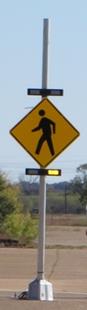
Figure 1. Photo. Study assembly containing LEDs above, below, and within the sign.

The location of the LEDs used in this study included the following:

• LEDs in rectangular beacons located above the sign. The bottom edge of the beacon housing was approximately 11.6 ft from the pavement.
  
  
• LEDs in rectangular beacons located below the sign. The bottom edge of the beacon housing was approximately 7.0 ft from the pavement.
  
  
• LEDs embedded within the sign. The height to the middle of the sign was approximately 9.5 ft.

Study Site

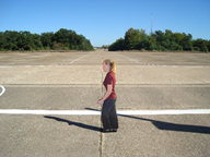
At the beginning of each participant run, the participants drove a Texas A&M Transportation Institute (TTI) vehicle to the study site (see figure 2) and parked the vehicle near the orange barrel (see figure 3 and figure 4). Figure 4 shows a photograph of the view for the participants. At the site, the participants saw two study assemblies: one on each side of the two-lane street. Vehicles were parked on the cross street upstream and downstream of the study site to aid in giving the urban feel and to provide a hiding space for the technicians that were changing the LED settings and moving the pedestrian cutout. Transverse white pavement crosswalk markings were installed at the site (see figure 5).

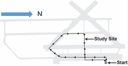
Figure 2. Illustration. Route for closed-course study.

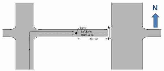
Figure 3. Illustration. Layout for the study site.

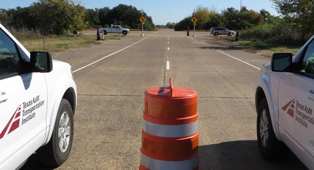
Figure 4. Photo. View of the study assemblies.

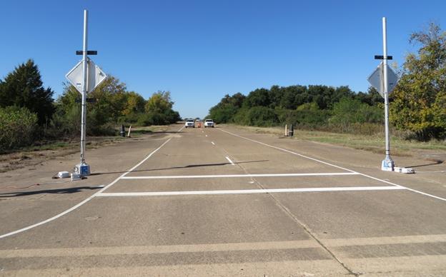
Figure 5. Photo. Back view of study site.

To be more efficient, the study was designed so that data were collected from two participants simultaneously. Each participant was in a unique car so that a participant's response would not be heard by the other participant. The vehicles were parked next to each other at the study site, thus simulating vehicles approaching a pedestrian crossing on a multilane roadway (see figure 3 and figure 4, which illustrate how the vehicles were parked). The participants were located 200 ft from the LED assemblies. The 200-ft distance was selected because it represents stopping sight distance (SSD) when traveling 30 mi/h.⁽³⁸⁾

Street lighting was present at the site for the nighttime testing. Two work zone light towers were rented for the study and placed on either side of the approach on the cross street. During course preparation, researchers positioned these light towers in a manner that simulated street lighting. Prior to collecting data for each set of nighttime participants, the luminance reading at the three pedestrian positions were taken to ensure a consistent street lighting level was present. The average of these readings was about 26 lux.

Cutout Pedestrian

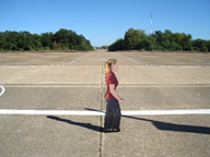
To ensure consistency with the pedestrian characteristics, the research team decided to use a photograph of a pedestrian. The photograph was cut out to mimic the shape of a walking pedestrian (see figure 6). Two cutouts were created to reflect two heights: adult and child. The 70-inch version reflected the average height of adults between 1999 and 2002, while the 54-inch version reflected the average height of a child in the same time period.⁽³⁹⁾ Figure 7 shows a researcher removing the short cutout photograph (center of road) after installing the tall cutout photograph (right side of road).

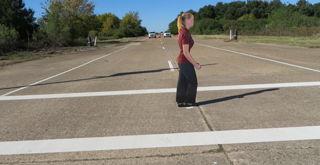
Figure 6. Photo. View of 54-inch cutout pedestrian used in study.

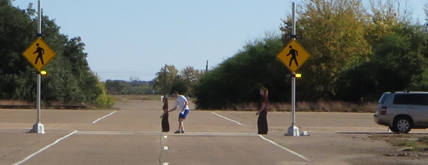
Figure 7. Photo. Researcher removing short cutout pedestrian after placing tall cutout pedestrian.

The cutout photographs were glued on both sides of a pole that extended a few inches below the shoe in the photograph. This extension was placed into one of three holes drilled into the pavement. The holes were located just to the right of the edgeline in the center of the road (i.e., on the lane line) and just to the left of the edgeline, as shown in figure 8. The positions near the edgeline pavement markings reflected the condition of a pedestrian waiting to cross the street. The center of the street represented a pedestrian in the crosswalk. The holes were drilled between the two crosswalk lines, as shown in figure 6 and figure 8. Because the photographs were glued to both sides of the pole, the cutout pedestrian could be rotated to appear to be walking to the left or to the right.

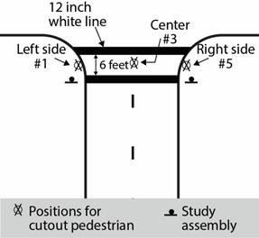
Figure 8. Illustration. Plan view showing pedestrian cutout positions.

Flash Pattern for Assemblies

Several flash patterns were used within the study. For the LEDs in rectangular beacons, the patterns shown in table 3 were used. The light bar containing the rectangular beacons had two unique beacons (with each beacon containing eight LEDs). When the beacon was turned on varied depending on the beacon location (i.e., left side or right side), as illustrated in table 3.

Table 3. Flash patterns used with LEDs located in rectangular beacons above or below the sign.

Cumulative Time (ms)	Sets I and II: No Flashes Dark		Set I: Wig-Wag Alternating		Sets I and II: 2-5 Flash Pattern		Set II: Two 125-ms Simultaneous Pulses
	Left Time On (ms)	Right Time On (ms)	Left Time On (ms)	Right Time On (ms)	Left Time On (ms)	Right Time On (ms)	Left Time On (ms)	Right Time On (ms)
0	0	0	25	0	25	0	25	25
25	0	0	25	0	25	0	25	25
50	0	0	25	0	25	0	25	25
75	0	0	25	0	25	0	25	25
100	0	0	25	0	25	0	25	25
125	0	0	25	0	0	0	0	0
150	0	0	25	0	0	0	0	0
175	0	0	25	0	0	0	0	0
200	0	0	25	0	25	0	25	25
225	0	0	25	0	25	0	25	25
250	0	0	25	0	25	0	25	25
275	0	0	25	0	25	0	25	25
300	0	0	25	0	25	0	25	25
325	0	0	25	0	0	0	0	0
350	0	0	25	0	0	0	0	0
375	0	0	25	0	0	0	0	0
400	0	0	25	0	0	25	0	0
425	0	0	25	0	0	0	0	0
450	0	0	25	0	0	25	0	0
475	0	0	25	0	0	0	0	0
500	0	0	0	25	0	25	0	0
525	0	0	0	25	0	0	0	0
550	0	0	0	25	0	25	0	0
575	0	0	0	25	0	0	0	0
600	0	0	0	25	0	25	0	0
625	0	0	0	25	0	25	0	0
650	0	0	0	25	0	25	0	0
675	0	0	0	25	0	25	0	0
700	0	0	0	25	0	25	0	0
725	0	0	0	25	0	25	0	0
750	0	0	0	25	0	25	0	0
775	0	0	0	25	0	25	0	0
800	0	0	0	25	BEC	BEC	BEC	BEC
825	0	0	0	25	BEC	BEC	BEC	BEC
850	0	0	0	25	BEC	BEC	BEC	BEC
875	0	0	0	25	BEC	BEC	BEC	BEC
900	0	0	0	25	BEC	BEC	BEC	BEC
925	0	0	0	25	BEC	BEC	BEC	BEC
950	0	0	0	25	BEC	BEC	BEC	BEC
975	0	0	0	25	BEC	BEC	BEC	BEC
Cycle length (ms)	N/A		1,000		800		800
Number of cycles/min	N/A		60		75		75

BEC = Beyond end of cycle.
N/A = Not applicable.
Note: Yellow shading represents when the beacons were on.

Table 4 shows the flash pattern used for the LEDs within the sign. While there are eight unique points of lights within an embedded diamond sign, the researchers decided that all eight LEDs would be illuminated at the same time within the sign as is currently used in practice. Therefore, there was not a left and right designation for the LEDs within the sign. The 2-5 flash pattern used with the assemblies was selected based on FHWA official interpretation 4(09)-21 (I) released on June 13, 2012, regarding the RRFB.⁽⁹⁾ It has two slower flashes on one side followed by five rapid flashes on other side.

Table 4. Flash patterns used with LEDs within sign.

Cumulative Time (ms)	Sets I and II: No Flashing	Set I: Five Pulses Similar to Right Side of RRFB	Sets I and II: One 100-ms Pulse	Set II: Two 125-ms Pulses Similar to Left Side of RRFB
	Time On (ms)	Time On (ms)	Time On (ms)	Time On (ms)
0	0	0	25	25
25	0	0	25	25
50	0	0	25	25
75	0	0	25	25
100	0	0	0	25
125	0	0	0	0
150	0	0	0	0
175	0	0	0	0
200	0	0	0	25
225	0	0	0	25
250	0	0	0	25
275	0	0	0	25
300	0	0	0	25
325	0	0	0	0
350	0	0	0	0
375	0	0	0	0
400	0	25	0	0
425	0	0	0	0
450	0	25	0	0
475	0	0	0	0
500	0	25	0	0
525	0	0	0	0
550	0	25	0	0
575	0	0	0	0
600	0	25	0	0
625	0	25	0	0
650	0	25	0	0
675	0	25	0	0
700	0	25	0	0
725	0	25	0	0
750	0	25	0	0
775	0	25	0	0
800	0	BEC	0	BEC
825	0	BEC	0	BEC
850	0	BEC	0	BEC
875	0	BEC	0	BEC
900	0	BEC	0	BEC
925	0	BEC	0	BEC
950	0	BEC	0	BEC
975	0	BEC	0	BEC
Cycle length (ms)	N/A	800	1,000	800
Number of cycles/min	N/A	75	60	75

N/A = Not applicable.
Note: Yellow shading represents when the beacons were on.

Brightness of LEDs

The characteristics of the LEDs may affect the detection of pedestrians. Table 5 lists the characteristics of the LEDs used with pattern set I, while table 6 provides similar values for pattern set II. To quantify the brightness of the pulsing lights, researchers used the photometric range within the TTI Visibility Laboratory. For each RRFB beacon and LED sign, a technician measured the 95th percentile peak intensity (called "measured intensity" in table 5 and table 6) and the optical power of the device. The researcher took the measurements at a vertical angle of 0 degrees and a horizontal angle of 0 degrees.

Peak luminous intensity is defined as the maximum luminous intensity for a given flash. The peak intensity can be much higher than the typical intensity within a pulse. Therefore, the 95th percentile intensity is used to provide a more representative value. The 95th percentile luminous intensity is the luminous intensity that 95 percent of the instantaneous intensity measurements are less than or equal to during the duration of the flash; instantaneous intensities measured during the dark period are not included in this measurement.

According to SAE Standard J595, optical power is defined as the integrated total of all flashes in a minute, in candela-s/min.⁽¹⁵⁾ Stated in a general way, optical power represents the area under the curve. It provides an appreciation of both the intensity of the pulses and the amount of time the LEDs are illuminated.

Table 5. LED characteristics for set I.

LED Location	Flash Pattern	Target Intensity (Candela)	Measured Intensity (Candela)	Optical Power (Candela-s/min)	Pulse Rate (Number of Pulses/Cycle Length)	On Ratio (Percent)
Above	2-5	600	622	25,600	8.75	69
Above	2-5	1,400	1,426	58,800	8.75	69
Above	2-5	2,200	2,207	91,000	8.75	69
Above	Wig-wag	600	605	36,300	2.00	100
Above	Wig-wag	1,400	1,442	86,500	2.00	100
Above	Wig-wag	2,200	2,237	134,200	2.00	100
Below	2-5	600	675	27,900	8.75	69
Below	2-5	1,400	1,450	59,800	8.75	69
Below	2-5	2,200	2,249	92,700	8.75	69
Below	Wig-wag	600	633	38,000	2.00	100
Below	Wig-wag	1,400	1,458	87,400	2.00	100
Below	Wig-wag	2,200	2,256	135,300	2.00	100
Within	100	600	649	3,900	1.00	10
Within	100	1,400	1,471	8,800	1.00	10
Within	100	2,200	2,225	13,300	1.00	10
Within	Five pulses	600	652	14,700	6.25	38
Within	Five pulses	1,400	1,454	32,700	6.25	38
Within	Five pulses	2,200	2,216	49,900	6.25	38

Note: Flash patterns are defined as follows: 2-5 = 2-5 flash pattern; wig-wag = wig-wag flash pattern; and 100 = one 100-ms flash pattern.

Table 6. LED characteristics for set II.

LED Location	Flash Pattern	Target Intensity (Candela)	Measured Intensity (Candela)	Optical Power (Candela-s/min)	Pulse Rate (Number of Pulses/Cycle Length)	On Ratio (Percent)
Above	125(2)	600	622	11,700	2.50	31
Above	125(2)	1,400	1,441	27,000	2.50	31
Above	125(2)	2,200	2,308	43,300	2.50	31
Above	2-5	600	622	25,600	8.75	69
Above	2-5	1,400	1,426	58,800	8.75	69
Above	2-5	2,200	2,207	91,000	8.75	69
Below	125(2)	600	619	11,600	2.50	31
Below	125(2)	1,400	1,436	26,900	2.50	31
Below	125(2)	2,200	2,269	42,500	2.50	31
Below	2-5	600	675	27,900	8.75	69
Below	2-5	1,400	1,450	59,800	8.75	69
Below	2-5	2,200	2,249	92,700	8.75	69
Within	100	600	652	3,900	1.00	10
Within	100	1,400	1,469	8,800	1.00	10
Within	100	2,200	2,227	13,400	1.00	10
Within	125(2)	600	646	12,100	2.50	31
Within	125(2)	1,400	1,464	27,400	2.50	31
Within	125(2)	2,200	2,227	41,800	2.50	31

Note: Flash patterns are defined as follows: 2-5 = 2-5 flash pattern; wig-wag = wig-wag flash pattern; 100 = one 100-ms flash pattern; and 125(2) = two 125-ms flashes.

Previous research has demonstrated that LED characteristics can influence whether an object is detected.⁽⁴⁰⁾ Because the amount of time the LEDs are on may influence a driver's ability to detect a pedestrian, a measure of the on time was developed. The on ratio variable (see table 5 and table 6) is defined to be the percentage of the 25-ms increments within a cycle where the LEDs within the beacon or sign are illuminated. The percentage of the cycle where the LEDs are dark would be determined as 1 minus the on ratio. For example, the 2-5 pattern would have an off ratio of 31 percent (100 percent - 69 percent). In the wig-wag pattern, there was no dark period, as demonstrated by having an on ratio of 100 percent. To provide an appreciation of how often the LEDs are pulsing, the pulse rate was determined as the number of pulses divided by the cycle length. For example, the 2-5 pattern had 7 pulses within the 0.8-s cycle for a pulse rate of 8.75, while the rapid-flashing LEDs within a sign had 5 pulses within the 0.8-s cycle for a pulse rate of 6.25.

Combinations Studied

The variables for participant characteristics and site characteristics presented within this closed-course study are as follows:

• Lighting: Day (natural lighting) or night (street lighting).
  
  
• Gender: Male or female.
  
  
• Age: Young (less than 55 years old) or old (55 years old or greater).
  
  
• Lane: Left lane or right lane.
  
  
• Viewing position: 200 ft upstream from assemblies.

Study assemblies characteristics included the following:

• LED location: LEDs in a rectangular beacon below the sign, LEDs in a rectangular beacon above the sign, or LEDs within the sign.
  
  
• Flash pattern (three per set; see table 3 and table 4):
  
  
  • Set I: No rectangular beacon above or below the sign, 2-5 pattern, or wig-wag (alternating) pattern.
    
    
  • Set I: No LEDs within the sign, five pulses (five pulses similar to the right side of the RRFB), or one 100-ms pulse (single pulse).
    
    
  • Set II: No rectangular beacon above or below the sign, 2-5 pattern, or two 125-ms pulses (simultaneous).
    
    
  • Set II: No LEDs within sign, five pulses (rapid right side of RRFB), or two 125-ms pulses (two pulses similar to left side of RRFB).
    
    
• Target intensity (i.e., brightness): 0, 600, 1,400, and 2,200 candelas.

The cutout pedestrian characteristics include the following:

• Pedestrian position: None, right side, center, or left side.
  
  
• Pedestrian height (when present): Tall (70 inches) or short (54 inches).
  
  
• Pedestrian direction (when present): Left or right.

Over 260 tests would be needed for a participant to see all possible combinations of study assembly and pedestrian characteristics. Preliminary data collection efforts demonstrated that about 100 tests could be conducted within the available 60-min data collection period.

A presentation order of the possible combinations between the study assembly and cutout pedestrian characteristics was developed using a random number generator in a spreadsheet. The order was then modified so that a participant would only see a particular combination once and so that a similar number of viewings per combination would occur. Table 7 shows the combinations tested. A total of 15 tests were conducted for each combination of pedestrian height and position. For example, the short cutout pedestrian when located in the center of the roadway was viewed in 15 tests. For the 7 combinations possible when considering pedestrian position and height, the 15 tests per combination resulted in a total of 105 tests per participant. For those tests when a cutout pedestrian was present (105 - 15 = 90 tests), half of the tests had the cutout pedestrian moving toward the left, while the other half of the tests had the cutout pedestrian moving toward the right.

Initially, the goal was to randomize the presentation order for all characteristics tested (i.e., LED location, flash pattern, brightness level, and cutout pedestrian position, height, and direction). Preliminary efforts demonstrated that the changes required of the technicians to switch from one LED location to another would consume too much time. Therefore, the study was subdivided into three blocks. Within the first block, all the tests associated with one of the LED locations would be conducted (e.g., rectangular below). A short break would be provided to the participant while the field crew switched the wires to operate the next LED location (e.g., LED within sign). Another break would divide the second block from the third block. Each block included 35 tests. The presentation of the device order was different for different sets of participants; some participants saw the above block first, some saw the below block first, and others saw the LED sign block first.

Table 7. Number of variable combinations tested during the closed-course study.

Location of LED	Flash Pattern	Target Intensity (Candela)	Number of Tests
			No Pedestrian Cutout Present	Short Pedestrian Cutout Position			Tall Pedestrian Cutout Position			Total
				Left Side	Center	Right Side	Left Side	Center	Right Side
Within	None	0	1	1	1			1	1	5
	Other	600	1	1	1	1	1			5
		1,400	1			1	1	1	1	5
		2,200	1	1	1	1		1		5
	Rapid	600		1	1		1	1	1	5
		1,400	1	1			1	1	1	5
		2,200	1	1	1	1			1	5
Below	None	0	1	1		1		1	1	5
	Other	600		1	1		1	1	1	5
		1,400	1		1		1	1	1	5
		2,200		1		1	1	1	1	5
	Rapid	600	1		1	1	1		1	5
		1,400	1	1		1	1	1		5
		2,200	1	1	1	1		1		5
Above	None	0	1		1	1	1		1	5
	Other	600			1	1	1	1	1	5
		1,400	1		1	1		1	1	5
		2,200	1	1	1		1		1	5
	Rapid	600		1		1	1	1	1	5
		1,400	1	1	1	1	1			5
		2,200		1	1	1	1	1		5
Grand Total			15	15	15	15	15	15	15	105

Note: Blank cells indicate that the combination was not tested.

Note that within the table, flash patterns are defined as follows:

• None: LEDs were not illuminated.
  
  
• Rapid: The 2-5 pattern was used when LEDs were above or below the sign, while five pulses (five pulses similar to the right side of the RRFB) were used when the LEDs were located within the sign.
  
  
• Other:
  
  
  • Set I: Wig-wag (alternating) was used when LEDs were above or below the sign, and a 100-ms pulse (single pulse) was used when LEDs were within the sign.
    
    
  • Set II: Two 125-ms pulses (simultaneous) were used when LEDs were above or below the sign, while two 125-ms pulses (two pulses similar to left side of RRFB) were used when LEDs were within the sign.

Concluding Survey

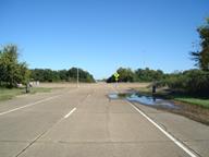
After participants completed the closed-course portion of the study, they were asked to complete a laptop survey that asked a series of queries to obtain the participants' opinions regarding flash patterns for beacons used with pedestrian crossing signs. The two initial queries included a video filmed from a driver's position as the vehicle moved toward a crosswalk with a waiting pedestrian. The participants always saw the same sign assembly; however, the LEDs and flash pattern used (if any) varied between the two queries. The same question was used with each query. Figure 9 shows the starting view for the first two queries (a close-up example of the sign assembly is shown in figure 1). The wording of the question and answers used with queries 1 and 2 are as follows:

As a driver of an automobile approaching the crosswalk shown in the video, how would you react in this situation?

1. I would slow and allow the pedestrian to cross the roadway.
   
   
2. I would stop and allow the pedestrian to cross the roadway.
   
   
3. I would confirm the pedestrian is not crossing before proceeding.
   
   
4. I would continue driving at the same speed.

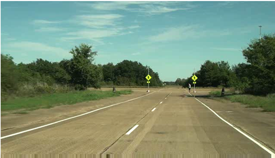
Figure 9. Photo. View at start of the driving video for the concluding survey for queries 1 and 2.

Researchers wanted to determine how drivers viewed the requirement to yield to the pedestrian when a pedestrian crossing sign did not have active supplemental LEDs. Therefore, the video for one of the two initial queries for all participants had no LEDs active (condition termed "sign" within the survey and is similar to the flash pattern "none" when wearing the occlusion glasses). About half of the participants had the sign-only video with their first query, while the other half of the participants had the sign-only video with their second query. Table 8 lists the videos shown for each query by participant group.

Table 9 identifies the flash pattern used with queries 1 and 2, which were the moving videos shown from a driver's perspective. Table 10 shows illustrations of the flash patterns used with queries 3 and 4, which were stationary videos showing a close-up of the pedestrian crossing assembly.

Table 8. Video assignments and flash patterns for each query by participant group.

Participant Group	Driving Video Flash Pattern		Stationary Video Flash Pattern
	Query 1	Query 2	Query 3		Query 4
	Video at Top of Screen	Video at Top of Screen	Video A at Left Side of Screen	Video B at Right Side of Screen	Video A at Left Side of Screen	Video B at Right Side of Screen
A	Sign	Below; 2-5	Within; 100	Below; 25(4)+200	Within; 125(2)	Below; 125(2)
B	Sign	Below; wig-wag	Below; 25(4)+200	Within; 25(4)+200	Sign	Within; 125(2)
C	Sign	Within; 100	Below; 25(4)+200	Within; 100	Below; 25(4)+200	Within; 125(2)
D	Below; 2-5	Sign	Below; 125(2)	Below; 2-5	Within; 25(4)+200	Within; 125(2)
E	Below; wig-wag	Sign	Within; 100	Within; 25(4)+200	Within; 100	Within; 125(2)
F	Within; 100	Sign	Within; 100	Below; 2-5	Sign	Within; 25(4)+200
G	Sign	Below; 2-5	Within; 125(2)	Within; 25(4)+200	Sign	Within; 100
H	Sign	Below; wig-wag	Sign	Below; 125(2)	Within; 25(4)+200	Sign
I	Sign	Within; 100	Below; 125(2)	Within; 25(4)+200	Below; 2-5	Sign
J	Below; 2-5	Sign	Within; 25(4)+200	Below; 125(2)	Below; 2-5	Within; 125(2)
K	Below; wig-wag	Sign	Below; 125(2)	Within; 100	Within; 25(4)+200	Below; 2-5
L	Within; 100	Sign	Within; 125(2)	Sign	Within; 125(2)	Within; 100
M	Sign	Below; 2-5	Below; 125(2)	Below; 25(4)+200	Below 25(4)+200	Below; 125(2)
N	Sign	Below; wig-wag	Below; 2-5	Within; 100	Within; 25(4)+200	Within; 100
O	Sign	Within; 100	Below; 2-5	Within; 25(4)+200	Within; 25(4)+200	Below; 25(4)+200
P	Below; 2-5	Sign	Below; 25(4)+200	Sign	Within; 100	Sign
Q	Below; wig-wag	Sign	Within; 125(2)	Below; 25(4)+200	Below; 2-5	Below; 25(4)+200
R	Within; 100	Sign	Sign	Below; 2-5	Within; 100	Below; 125(2)
S	Sign	Below; 2-5	Below; 125(2)	Sign	Within; 125(2)	Below; 2-5
T	Sign	Below; wig-wag	Sign	Below; 25(4)+200	Below; 25(4)+200	Below; 2-5
U	Sign	Within; 100	Below; 2-5	Below; 125(2)	Below; 125(2)	Within; 125(2)

Note: Flash patterns are defined as follows: sign = no active LEDs; 2-5 = 2-5 flash pattern; wig-wag = wig-wag flash pattern; 100 = one 100-ms flash pattern; 25(4)+200 = four 25-ms flashes and one 200-ms flash; and 125(2) = two 125-ms flashes.

Table 9. Flash patterns for queries 1 and 2 showing moving videos from driver perspective.

Cumulative Time (ms)	Below; Wig-Wag Flash Pattern		Below; 2-5 Flash Pattern		Within; 100-ms Flash Pattern	No LEDs or Flash Pattern
	Left Time On (ms)	Right Time On (ms)	Left Time On (ms)	Right Time On (ms)	Time On (ms)	Time On (ms)
0	25	0	25	0	25	0
25	25	0	25	0	25	0
50	25	0	25	0	25	0
75	25	0	25	0	25	0
100	25	0	25	0	0	0
125	25	0	0	0	0	0
150	25	0	0	0	0	0
175	25	0	0	0	0	0
200	25	0	25	0	0	0
225	25	0	25	0	0	0
250	25	0	25	0	0	0
275	25	0	25	0	0	0
300	25	0	25	0	0	0
325	25	0	0	0	0	0
350	25	0	0	0	0	0
375	25	0	0	0	0	0
400	25	0	0	25	0	0
425	25	0	0	0	0	0
450	25	0	0	25	0	0
475	25	0	0	0	0	0
500	0	25	0	25	0	0
525	0	25	0	0	0	0
550	0	25	0	25	0	0
575	0	25	0	0	0	0
600	0	25	0	25	0	0
625	0	25	0	25	0	0
650	0	25	0	25	0	0
675	0	25	0	25	0	0
700	0	25	0	25	0	0
725	0	25	0	25	0	0
750	0	25	0	25	0	0
775	0	25	0	25	0	0
800	0	25	BEC	BEC	BEC	0
825	0	25	BEC	BEC	BEC	0
850	0	25	BEC	BEC	BEC	0
875	0	25	BEC	BEC	BEC	0
900	0	25	BEC	BEC	BEC	0
925	0	25	BEC	BEC	BEC	0
950	0	25	BEC	BEC	BEC	0
975	0	25	BEC	BEC	BEC	0

Note: Yellow shading represents when the beacons were on.

Table 10. Flash patterns used for queries 3 and 4 with the video showing a close-up view.

Cumulative Time (ms)	Below; 2-5 Flash Pattern		Below; Two 125-ms Flashes		Below; Four 25-ms Flashes and One 200-ms Flash		Within; 100-ms Flash Pattern	Within; Two 125-ms Flashes	Within; Four 25-ms Flashes and One 200-ms Flash	No Flash Pattern
	Left Time On (ms)	Right Time On (ms)	Left Time On (ms)	Right Time On (ms)	Left Time On (ms)	Right Time On (ms)	Time On (ms)	Time On (ms)	Time On (ms)	Time On (ms)
0	25	0	25	25	0	0	25	25	0	0
25	25	0	25	25	0	0	25	25	0	0
50	25	0	25	25	0	0	25	25	0	0
75	25	0	25	25	0	0	25	25	0	0
100	25	0	25	25	0	0	0	25	0	0
125	0	0	0	0	0	0	0	0	0	0
150	0	0	0	0	0	0	0	0	0	0
175	0	0	0	0	0	0	0	0	0	0
200	25	0	25	25	0	0	0	25	0	0
225	25	0	25	25	0	0	0	25	0	0
250	25	0	25	25	0	0	0	25	0	0
275	25	0	25	25	0	0	0	25	0	0
300	25	0	25	25	0	0	0	25	0	0
325	0	0	0	0	0	0	0	0	0	0
350	0	0	0	0	0	0	0	0	0	0
375	0	0	0	0	0	0	0	0	0	0
400	0	25	0	0	25	25	0	0	25	0
425	0	0	0	0	0	0	0	0	0	0
450	0	25	0	0	25	25	0	0	25	0
475	0	0	0	0	0	0	0	0	0	0
500	0	25	0	0	25	25	0	0	25	0
525	0	0	0	0	0	0	0	0	0	0
550	0	25	0	0	25	25	0	0	25	0
575	0	0	0	0	0	0	0	0	0	0
600	0	25	0	0	25	25	0	0	25	0
625	0	25	0	0	25	25	0	0	25	0
650	0	25	0	0	25	25	0	0	25	0
675	0	25	0	0	25	25	0	0	25	0
700	0	25	0	0	25	25	0	0	25	0
725	0	25	0	0	25	25	0	0	25	0
750	0	25	0	0	25	25	0	0	25	0
775	0	25	0	0	25	25	0	0	25	0

Note: Yellow shading represents when the beacons were on.

Queries 3 and 4 asked the participants to judge the urgency of the message conveyed by the crosswalk treatment. The participants saw a close-up of two side-by-side assemblies labeled video A and video B. The flash patterns and which LEDs were active varied, as listed in table 8. The design of the study resulted in four to five participants seeing each pair with the specific placement on the screen (i.e., left side or right side). If placement on the screen was not considered, then each device pair was viewed, on average, by nine participants. The wording of the question and answers used with queries 3 and 4 were as follows:

In your opinion, which video conveys a more urgent need for a driver to yield to a pedestrian?

1. Video A conveys a more urgent need.
   
   
2. Video B conveys a more urgent need.
   
   
3. The level of urgency is similar in both videos.
   
   
4. Neither video conveys an urgent need for a driver to yield to a pedestrian.

The final query asked the participants to count how many flashes they observed in the left and right beacons for a light bar that was located in the room with them.

DATA COLLECTION

Study Periods

The study was conducted under both daytime and nighttime conditions between Wednesday, November 13, 2013, and Thursday, December 12, 2013, with several days lost due to rain. Sunset occurred at approximately 5:30 p.m. during the study. The study took about 1.5 h from meeting the participant to the participant receiving their payment. About one-third of the participants drove during daylight hours, and two-thirds drove during nighttime conditions with an approximately even split between flash pattern sets I and II. The following start times were used:

• 12 p.m.
  
  
• 1:30 p.m.
  
  
• 6:30 p.m.
  
  
• 8 p.m.

Participants

Participants were recruited from the area using TTI's pool of previous research subjects list. Over the phone, the potential participants were told that the study was confidential and the records of the study would be kept private. They were also told that their participation was voluntary and that they were free to withdraw from the study at any time.

The initial intent was to recruit a group of participants composed of one-quarter males over the age of 55, one-quarter females over the age of 55, one-quarter males under the age of 55, and one-quarter females under the age of 55. Within each of those demographic groups, the goal was to have an even distribution between those who participated during the daytime and nighttime within pattern set I. Therefore, the following divisions were used in structuring participant recruitment:

• Light level: Day or night.
  
  
• Age group: Young (younger than 55 years old) and old (55 years old or older).
  
  
• Gender: Male or female.

When pattern set II was added to the study, data were only collected during the nighttime.

The male/female, young/old divisions resulted in four participant categories. The research goal was to have 8 participants in each of these categories, resulting in 32 participants per day or per night. Table 11 summarizes the number of participants by pattern set (I or II) and light level (day or night) that participated in the study.

Participants were at least 18 years old and possessed a valid driver's license with no restrictions. Upon completion of the survey, participants received monetary compensation of $50.

Table 11. Distribution of participants.

Day or Night	Pattern Set	Old Female	Old Male	Old Total	Young Female	Young Male	Young Total	Young Total
Day	I	9	8	17	8	7	15	32
Night	I	8	7	15	8	9	17	32
Night	II	8	8	16	9	9	18	34
Grand Total		25	23	48	25	25	50	98

Participant's Tasks

The tasks for the participants for this closed-course study were as follows:

1. After vision was restored by the occlusion glasses, participants were asked to indicate via a button push whether the pedestrian was walking to the left or to the right.
   
   
2. Following the driver's identification of the pedestrian direction, participants were asked to state whether the intensity of the LEDs was comfortable, irritating, or unbearable.
   
   
3. Participants responded to survey queries presented in a conference room at the conclusion of the study.

Instrumented Vehicle

Two similar vehicles—2009 sports utility vehicles—served as the participant cars for this experiment. The headlamps for these vehicles were 35 inches from the ground and 27 inches from center of the vehicle. Prior to the start of the study, the headlamps on both vehicles were properly aligned by TTI staff members.

Participant Intake

Participant intake was headquartered at TTI's Environmental Emissions Research Facility on the Riverside campus. This location was selected because it was near the driving route, had public parking available, included restroom facilities, and was available for both daytime and nighttime use during the data collection period. After meeting with a member of the research team to review the informed consent documentation and complete the demographic questionnaire, participants were given an overview of the study, including how the data were to be collected. They were also given a Dvorine color vision test.

To ensure consistency, the research team used scripts and slide shows to aid in providing instructions to each participant. The script used during intake was as follows:

"Now, let me tell you a little about your tasks. There are two parts. For the first part, you will be driving a State-owned passenger vehicle on a closed course we have set up on airport runways, taxiway, and roadways here at the Riverside campus. The vehicle is specially equipped to record and measure various driving characteristics, but drives just like a normal car. A researcher will be in the car with you at all times and will direct you when, where, and how fast you will need to go. The fastest you will be asked to drive is 40 mi/h.

For one part, you will be driving a course marked with white and yellow striping just as you would see on an actual road. Part of the route is not striped, and when we reach these segments, I will point you to the reflective pavement markings/line in the pavement that will act as our road's "center line." Once we arrive to the study location, we will ask you to park your vehicle next to the orange barrels. There will be another participant in a vehicle next to you. We are running two participants simultaneously to more efficiently collect data for this study.

Once the vehicle is in position we will ask you to place it into park. We will then ask you to place the occlusion glasses over your eyes and glasses if you have glasses. The occlusion glasses will block your vision until the start of the test. When you are ready, we will clear the occlusion glasses and restore your vision. You are to tell us via a button push whether the pedestrian in the downstream crosswalk is walking to the left, to the right, or is not present. We will practice the button pushes prior to driving to the study sites. After you indicate which way the pedestrian is walking, I will ask you to indicate if the beacon glare is comfortable, irritating, or unbearable.

• Comfortable (where the glare is not annoying and the signal is easy to look at).
  
  
• Irritating (where the glare is uncomfortable, however you are still able to look at it without the urge to look away).
  
  
• Unbearable (where the glare is so intense that you want to avoid looking at it).

After completing the tests you will return here for a brief laptop survey. After the laptop survey we will provide your payment."

Initial Button Push Training

As part of the intake process, the participants practiced with a button box while responding to photographs of the crossing. The objectives for this part of the study were as follows:

• Train participants to recognize the pedestrians as well as absence of the pedestrians.
  
  
• Provide the opportunity for the participants to become familiar with using three buttons to record their responses.

During the training tests, the participant pressed a button when they determined the direction the pedestrian was walking. Because of the software used for this test and available response pads for this software, the button box used for this training had seven buttons. Figure 10 through figure 12 show three of the photos along with the accompanying instructions used in the initial training. A random mix of tall and short cutout pedestrians moving to the right and to the left and in positions 1, 3, or 5 (illustrated in figure 8) were used within the training.

When the pedestrian in the crosswalk is moving to the left (as shown) please press (3) (do so now).

Figure 10. Photo. Training example with pedestrian facing left.

When the pedestrian in the crosswalk is moving to the right (as shown) please press (5) (do so now).

Figure 11. Photo. Training example with pedestrian facing right.

When no pedestrian is present in the crosswalk (as shown) please press (4) (do so now).

Figure 12. Photo. Training example with no pedestrian.

Vehicle Review

Participants were escorted to the TTI vehicle and given a walk-through of the vehicle's features. They were provided with the opportunity to adjust the seat and mirrors and to become accustomed to the controls of the vehicle.

Participants were informed that they would drive the vehicle on a closed course and were told to drive at a speed not exceeding 40 mi/h on the runways. They were asked to drive the runway system as though it was a regular roadway and were reminded that they had complete control of the vehicle at all times. A researcher accompanied the participant in the back seat, controlling the data collection equipment and providing direction. Participants were told to keep the vehicle's headlamps on the low setting if testing at night. They were told to drive to the study site and to position the vehicle by the barrel. Once in position, they were told to place the vehicle into park.

Data Collection at Study Site

At the study site, the participants were reminded that they would be wearing occlusion glasses that would block their vision until the start of the test and that they would provide responses via a three-button box within the vehicle. The researcher handed the participant the button box and asked them to become acquainted with the button box and to determine how best to hold the box comfortably in their hands. When the participant indicated they were comfortable with the box, they were provided the occlusion glasses, which they placed on their face over their eyeglasses if they were wearing any.

After the participants indicated that the glasses and button box were comfortable, the practice testing began for at least three scenarios. After the practice, the testing began. When the participant had indicated readiness and the field crew indicated readiness for the cutout pedestrian and study assembly, the researcher cleared the glasses and restored vision. The participants were then asked to indicate via a pushbutton whether the pedestrian in the downstream crosswalk was walking to the left or to the right or whether the pedestrian was not present.

The participants were provided the following instruction in case they felt the brightness was too bright for them:

If you find the brightness level of the beacons to be agonizing and you are not comfortable completing the task for a particular test, please look away from the crosswalk and tell me. I will block your vision for that test and will radio the field crew to setup for the next test.

After the participants pushed a button on the button box, which would darken the glasses, they were to provide their rating of the brightness of the lights on the traffic control device. The three rating levels used were as follows:

• Comfortable: The glare was not annoying, and the signal was easy to look at.
  
  
• Irritating: The glare was uncomfortable; however, participants could still look at it without the urge to look away.
  
  
• Unbearable: The glare was so intense that participants wanted to avoid looking at it.

After the participants indicated the rating level, the researcher radioed the field crew and told them to set up for the next test. This process was repeated until the participants had completed all the tests at the site.

The participants were also provided these additional instructions:

If at any point in time you wish to stop, or would like a break, let me know and we will stop or allow you an opportunity to rest.

Please leave the vehicle in park during these tests and while you are wearing the occlusion glasses.

DATA REDUCTION

Participant Demographics

Table 12 lists the demographic information for the 98 participants. The large number that selected retired for employment (34 percent) is a reflection of the emphasis on having half of the drivers over 55 years old.

Table 12. Demographic information for participants.

Characteristic		Set I, Day		Set I, Night		Set II, Night		Total
		Number	Percent	Number	Percent	Number	Percent	Number	Percent
Gender	Female	17	53	16	50	17	50	50	51
	Male	15	47	16	50	17	50	48	49
Age group	< 55 years old	17	53	15	47	16	47	48	49
	≥ 55 years old	15	47	17	53	18	53	50	51
Employment	Full time	11	34	12	37	13	38	36	37
	Part time	4	13	2	6	4	12	10	10
	Retired	13	41	10	31	10	29	33	34
	Student/part time	1	3	4	13	5	15	10	10
	Other	3	9	4	13	2	6	9	9
Miles driven per year	< 10,000 mi	5	16	5	16	6	18	16	16
	10,000-15,000 mi	14	44	14	44	15	44	43	44
	> 15,000 mi	13	41	13	41	13	38	39	40
Normal driving conditions	Rural roads	9	28	7	22	11	32	27	28
	City streets	15	47	16	50	12	35	43	44
	Freeways	1	3	3	9	0	0	4	4
	Mixed	7	22	6	19	11	32	24	24

Data Cleaning

Before proceeding with the statistical analyses, the data were reviewed to identify and remove tests that needed to be eliminated due to miscoded information regarding the response type, the wrong LEDs being activated in the assembly, or incorrect pedestrian size, position, or direction. In a few cases, participants would self-correct a button push. To have all response times only reflect initial reactions, the detection time results for a given test with duplicate responses were eliminated. These data were included in the detection accuracy evaluations. Instances where animals crossed in front of the vehicles were eliminated as well.

Responses

The computer software program along with the response pad unit were used to record the time between the occlusion glasses being cleared and the participants pressing a button in the response pad. These data were recorded within a spreadsheet that contained an experiment label, a time stamp, and the corresponding detection time. For each experiment, the researcher asked about the glare immediately after each participant pressed a button in the response pad. The experimenters manually recorded discomfort glare ratings using preprinted data sheets.

Each of the experiment labels corresponded to predetermined combinations of pedestrian height, position, brightness, and flash pattern. The sequence of experiments was random within the blocking structure described previously in this report. The spreadsheet with detection time data was later combined with the corresponding experiment conditions and discomfort data per experiment label.

Box Plots

For some analyses, results were presented visually in the form of box plots or quantitatively in the form of statistical analysis. Box plots presented in this report were generated using the convention that the central line in the box represents the median data point (see figure 13). The top of the box represents the 75th percentile, and the bottom represents the 25th percentile. Thus, the relative position of the median score within the 75th and 25th percentiles can give some indication about the skewness of the data. The height of the box is known as the "interquartile range" (IQR). The "whiskers" represent the data that lie 1.5 times beyond the IQR. If all data below the 25th percentile and above the 75th percentile are within 1.5 times the IQR, then the end of the whisker represents the greatest or smallest value. Otherwise, all outliers beyond 1.5 times the IQR, added or subtracted from the 25th and 75th percentiles, respectively, are plotted using small black open circles.

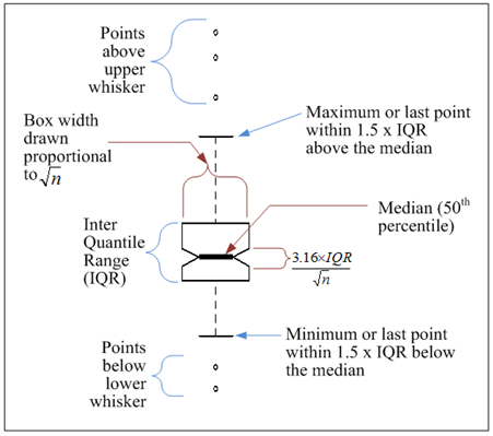
Figure 13. Illustration. Box plot details.

Additionally, it should be noted that a box plot representing a large sample provides more confidence on its quartiles than another box plot representing a smaller sample. For this reason, when two or more box plots are drawn together, the following two metrics of sample sizes are represented:

• The box plot width is drawn proportional to the square root of the sample size, n.
  
  
• A triangular notch is symmetrically cut around the median and has a total width of. This feature allows a preliminary graphic assessment of differences of medians, since such notch width has been proposed to roughly represent a 95 percent confidence interval around the median.⁽⁴¹⁾ For example, two medians are significantly different if the notches of two box plots do not overlap, but nothing can be said (that is, preliminarily) if there is overlap between notches.

Mosaic Plots

For some analyses, results were presented visually in the form of mosaic plots. Mosaic plots divide each dimension of a rectangular space in sizes relative of the levels of a variable assigned to that dimension. Thus, this type of plot can represent two variables at the time, where each variable may have two or more levels. Figure 14 shows the details of a mosaic plot when the variable assigned to the height is the number of correct/incorrect pedestrian detections.

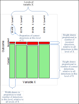
Figure 14. Illustration. Mosaic plot details.

Potential Outliers

Preliminary statistical analyses were examined for outlying data points in the fit. Data points identified in this way were tested for their impact on the analysis. Most of the cases identified in this stage came from a young participant with distinctive fast detection times and high accuracy in the daytime dataset. The data from this participant were identified in the analysis stage. The analysis was tested for sensitivity to this subset, but it was verified that the conclusions remained virtually unchanged, with or without these data. For robustness, results in this report include the data from this participant.

FINDINGS

Detection Time to Correctly Identify Pedestrian Walking Direction

During the daytime, the average detection time to pedestrian direction was 1,137 ms from a sample of 2,998 correct detections. At night, the average detection time was notably longer—1,376 ms from a sample of 6,091 correct detections. This roughly represents a 25 percent increase in detection time at night. Table 13 shows the average detection time for the daytime data, while table 14 provides the nighttime average detection time for pattern set I. Nighttime average detection time for pattern set II is in table 15 along with nighttime average for both pattern sets I and II.

Table 13. Daytime average detection time for set I.

Target Intensity (Candela)	Flash Pattern	Location of LED	Older Participants		Younger Participants		Combined Participants
			Number of Participants	Average Detection Time (ms)	Number of Participants	 Average Detection Time (ms)	Number of Participants	Average Detection Time (ms)
600	100	Within	70	1,356	66	967	136	1,167
600	Five pulses	Within	73	1,170	65	1,015	138	1,097
600	2-5	Above	71	1,219	70	929	141	1,075
600	2-5	Below	82	1,336	63	1,068	145	1,220
600	Wig-wag	Above	74	1,197	70	907	144	1,056
600	Wig-wag	Below	81	1,200	63	963	144	1,096
1,400	100	Within	72	1,311	66	972	138	1,149
1,400	Five pulses	Within	73	1,211	67	968	140	1,095
1,400	2-5	Above	76	1,339	70	979	146	1,166
1,400	2-5	Below	82	1,276	62	969	144	1,144
1,400	Wig-wag	Above	75	1,318	70	960	145	1,145
1,400	Wig-wag	Below	79	1,247	65	938	144	1,107
2,200	100	Within	75	1,311	67	1,013	142	1,170
2,200	Five pulses	Within	74	1,286	68	972	142	1,136
2,200	2-5	Above	79	1,291	69	966	148	1,140
2,200	2-5	Below	81	1,566	62	1,065	143	1,349
2,200	Wig-wag	Above	77	1,333	70	912	147	1,132
2,200	Wig-wag	Below	81	1,332	62	1,025	143	1,199
None	Sign	Above	71	1,190	69	910	140	1,052
None	Sign	Below	83	1,240	65	985	148	1,128
None	Sign	Within	72	1,145	68	940	140	1,046
Total			1,601	1,281	1,397	971	2,998	1,137

Note: Flash patterns are defined as follows: 100 = one 100-ms flash pattern; 2-5 = 2-5 flash pattern; wig-wag = wig-wag flash pattern; and sign = no active LEDs.

Table 14. Nighttime average detection time for set I.

Target Intensity (Candela)	Flash Pattern	Location of LED	Older Participants		Younger Participants		Combined Participants
			Number of Participants	Average Detection Time (ms)	Number of Participants	Average Detection Time (ms)	Number of Participants	Average Detection Time (ms)
600	100	Within	70	1,781	81	1,106	151	1,419
600	Five pulses	Within	67	1,609	83	1,120	150	1,338
600	2-5	Above	69	1,525	83	1,208	152	1,352
600	2-5	Below	65	1,700	79	1,270	144	1,464
600	Wig-wag	Above	72	1,654	79	1,215	151	1,424
600	Wig-wag	Below	71	1,900	80	1,459	151	1,666
1,400	100	Within	69	1,609	80	1,184	149	1,380
1,400	Five pulses	Within	70	1,596	84	1,147	154	1,351
1,400	2-5	Above	68	1,511	81	1,237	149	1,362
1,400	2-5	Below	68	1,822	79	1,527	147	1,663
1,400	Wig-wag	Above	67	1,495	78	1,240	145	1,358
1,400	Wig-wag	Below	61	1,870	76	1,520	137	1,676
2,200	100	Within	70	1,526	85	1,098	155	1,291
2,200	Five pulses	Within	67	1,603	81	1,231	148	1,399
2,200	2-5	Above	67	1,623	82	1,298	149	1,444
2,200	2-5	Below	61	1,706	75	1,363	136	1,517
2,200	Wig-wag	Above	71	1,745	78	1,277	149	1,500
2,200	Wig-wag	Below	57	2,567	71	1,979	128	2,241
None	Sign	Above	68	1,345	83	1,173	151	1,250
None	Sign	Below	70	1,747	83	1,184	153	1,442
None	Sign	Within	70	1,500	84	1,059	154	1,260
Grand Total			1,418	1,680	1685	1,274	3,103	1,459

Note: Flash patterns are defined as follows: 100 = one 100-ms flash pattern; 2-5 = 2-5 flash pattern; wig-wag = wig-wag flash pattern; and sign = no active LEDs.

Table 15. Nighttime average detection time for set II and combined total for sets I and II.

Target Intensity (Candela)	Flash Pattern	Location of LED	Older Participants		Younger Participants		Combined Participants
			Number of Participants	Average Detection Time (ms)	Number of Participants	Average Detection Time (ms)	Number of Participants	Average Detection Time (ms)
600	100	Within	70	1,227	72	1,257	142	1,242
600	125(2)	Above	69	1,167	72	1,192	141	1,179
600	125(2)	Below	66	1,195	72	1,246	138	1,221
600	125(2)	Within	69	1,132	76	1,311	145	1,226
600	2-5	Above	71	1,254	77	1,262	148	1,258
600	2-5	Below	61	1,558	76	1,383	137	1,461
1,400	100	Within	67	1,218	75	1,350	142	1,287
1,400	125(2)	Above	69	1,170	76	1,322	145	1,250
1,400	125(2)	Below	73	1,236	73	1,302	146	1,269
1,400	125(2)	Within	69	1,191	72	1,327	141	1,260
1,400	2-5	Above	68	1,249	78	1,303	146	1,278
1,400	2-5	Below	63	1,479	74	1,451	137	1,464
2,200	100	Within	71	1,202	74	1,242	145	1,222
2,200	125(2)	Above	72	1,191	79	1,312	151	1,255
2,200	125(2)	Below	68	1,394	71	1,343	139	1,368
2,200	125(2)	Within	67	1,320	74	1,470	141	1,399
2,200	2-5	Above	66	1,304	78	1,412	144	1,362
2,200	2-5	Below	50	1,390	75	1,481	125	1,445
None	Sign	Above	67	1,224	80	1,158	147	1,188
None	Sign	Below	67	1,385	76	1,214	143	1,294
None	Sign	Within	72	1,189	73	1,217	145	1,203
Total Set II			1,415	1,265	1573	1,312	2,988	1,290
Combined Total Sets I and II			2,833	1,473	3258	1,292	6,091	1,376

Note: Flash patterns are defined as follows: 100 = one 100-ms flash pattern; 125(2) = two 125-ms flashes; 2-5 = 2-5 flash pattern; and sign = no active LEDs

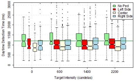
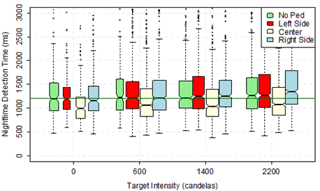
Box plots were generated to demonstrate trends in the data before conducting the formal statistical analysis. The plots in figure 15 for daytime and figure 16 for nighttime demonstrate that detection time tended to be shorter for lower intensity and longer for higher intensity regardless of the location of the LEDs. This trend was more obvious at night (see figure 16). The trends held even when the data were sorted by pedestrian position rather than LED locations (see figure 17 for daytime and figure 18 for nighttime). The groups of boxes clearly tend to be higher to the right of the plot, which corresponds to higher intensities.

Figure 17 and figure 18 demonstrate a clear trend regarding the pedestrian position in the crosswalk. The time to correctly identify that there was no pedestrian in the crosswalk appears similar at different levels of LED intensity and at day and nighttime (i.e., the green boxes). The median detection time for that case was about 1,200 ms (i.e., the added horizontal line in the plots). In all other correct responses, it is clear that nighttime had longer times, but the relative trends appear constant; a pedestrian at the center of the crosswalk triggered faster detections than either pedestrian at the right or the left side of the crosswalk.

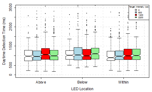
Figure 15. Graph. Daytime detection time by LED location and target intensity.

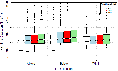
Figure 16. Graph. Nighttime detection time by LED location and target intensity.

Note: The horizontal line represents the median detection time.

Figure 17. Graph. Daytime detection time by pedestrian position and target intensity.

Note: The horizontal line represents the median detection time with no pedestrian present.

Figure 18. Graph. Nighttime detection time by pedestrian position and target intensity.

It should be noted that the plots make evident the fact that the data are heavily skewed toward longer detection times, especially at night. This means that the data are more disperse at values above the median than below the median. To control for this characteristic, the statistical analysis was performed using the natural logarithm of the detection time. This data transformation reduced the skewness while preserving the percentile ranks in the data. More details are provided in the Statistical Analysis section in this chapter.

Accuracy of Detecting Pedestrian Direction

Accuracy of detecting pedestrian direction was determined by the number of participants who correctly detected the direction of the cutout pedestrian to the number of participants for the given characteristics (e.g., flash pattern, etc.). Table 16 shows the accuracy rate for daytime, while table 17 shows similar data for nighttime. During the daytime, the average rate of correct detections of pedestrian direction was 98 percent from a sample of 3,053 detections. At night, the average detection rate was notably lower, 93 percent, from a sample of 6,515 detections.

Table 16. Daytime accuracy of correct detection for set I.

Target Intensity (Candela)	Flash Pattern	Location of LED	Older Participant Accuracy (Percent)	Younger Participant Accuracy (Percent)	All Participant Accuracy (Percent)	Sample Size
600	Five pulses	Within	99	98	99	140
600	Wig-wag	Above	93	100	96	150
600	Wig-wag	Below	95	98	97	149
600	100	Within	95	99	96	141
600	2-5	Above	97	100	99	143
600	2-5	Below	96	100	98	148
1,400	Five pulses	Within	99	100	99	141
1,400	Wig-wag	Above	96	100	98	148
1,400	Wig-wag	Below	98	100	99	146
1,400	100	Within	99	99	99	140
1,400	2-5	Above	97	100	99	148
1,400	2-5	Below	99	98	99	146
2,200	Five pulses	Within	100	100	100	142
2,200	Wig-wag	Above	100	100	100	147
2,200	Wig-wag	Below	95	97	96	149
2,200	100	Within	99	100	99	143
2,200	2-5	Above	99	99	99	150
2,200	2-5	Below	96	97	97	148
None	Sign	Above	96	100	98	143
None	Sign	Below	98	100	99	150
None	Sign	Within	99	100	99	141
Grand Total			97	99	98	3,053

Note: Flash patterns are defined as follows: wig-wag = wig-wag flash pattern; 100 = one 100-ms flash pattern; 2-5 = 2-5 flash pattern; and sign = no active LEDs.

Table 17. Nighttime accuracy of correct detection.

Target Intensity (Candela)	Flash Pattern	Location of LED	Set I		Set II		All Participant Accuracy (Percent)	Sample Size
			Older Participant Accuracy (Percent)	Younger Participant Accuracy (Percent)	Older Participant Accuracy (Percent)	Younger Participant Accuracy (Percent)
600	Five pulses	Within	89	98	NS	NS	94	160
600	Wig-wag	Above	99	98	NS	NS	98	154
600	Wig-wag	Below	95	95	NS	NS	95	159
600	100	Within	93	98	93	91	94	312
600	125(2)	Above	NS	NS	92	92	92	153
600	125(2)	Below	NS	NS	90	92	91	151
600	125(2)	Within	NS	NS	92	96	94	154
600	2-5	Above	93	100	96	99	97	309
600	2-5	Below	87	95	84	95	90	311
1,400	Five pulses	Within	93	100	NS	NS	97	159
1,400	Wig-wag	Above	96	98	NS	NS	97	150
1,400	Wig-wag	Below	84	89	NS	NS	87	158
1,400	100	Within	92	98	92	96	94	308
1,400	125(2)	Above	NS	NS	92	96	94	154
1,400	125(2)	Below	NS	NS	99	94	96	152
1,400	125(2)	Within	NS	NS	92	96	94	150
1,400	2-5	Above	91	98	93	99	95	310
1,400	2-5	Below	91	94	85	93	91	313
2,200	Five pulses	Within	89	95	NS	NS	93	160
2,200	Wig-wag	Above	97	96	NS	NS	97	154
2,200	Wig-wag	Below	78	85	NS	NS	82	157
2,200	100	Within	93	100	95	95	96	313
2,200	125(2)	Above	NS	NS	96	99	97	155
2,200	125(2)	Below	NS	NS	92	92	92	151
2,200	125(2)	Within	NS	NS	89	95	92	153
2,200	2-5	Above	91	98	90	98	94	311
2,200	2-5	Below	82	89	71	94	85	308
None	Sign	Above	92	100	89	100	96	312
None	Sign	Below	95	100	92	95	95	310
None	Sign	Within	93	99	96	92	95	314
Grand Total			91	96	91	95	93	6,515

Note: Flash patterns are defined as follows: wig-wag = wig-wag flash pattern; 100 = one 100-ms flash pattern; 125(2) = two 125-ms flashes; 2-5 = 2-5 flash pattern; and sign = no active LEDs.
NS = Flash pattern was not studied within the set.

Mosaic plots were generated to demonstrate trends in the data before conducting a formal statistical analysis. The plots in figure 19 and figure 20 demonstrate that the percent of correct detections tends to be lower for higher target intensity at night. This trend is not seen in the daytime data.

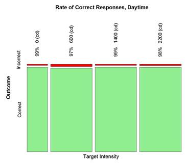
Figure 19. Graph. Daytime correct detection rate by target intensity.

>

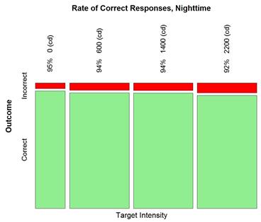
Figure 20. Graph. Nighttime correct detection rate by target intensity.

Figure 21 and figure 22 demonstrate that when subdividing the data by flash pattern, no trend appeared clear for daytime. It appears that the 2-5 (rapid) and wig-wag patterns tended to have slightly lower correct detection rates than the rest of patterns for nighttime condition.

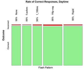
Figure 21. Graph. Daytime correct detection rate by flash pattern.

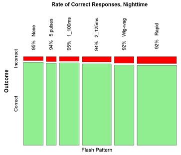
Figure 22. Graph. Nighttime correct detection rate by flash pattern.

Finally, the trends by age are demonstrated by figure 23 for daytime and figure 24 for nighttime. It seems clear the older participants tended to be less accurate than young participants.

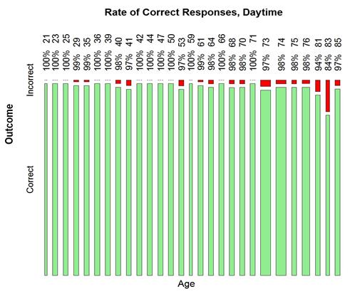
Figure 23. Graph. Daytime detection rate by age.

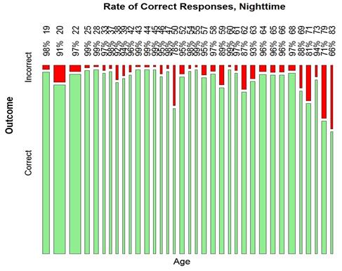
Figure 24. Graph. Nighttime detection rate by age.

Discomfort

After the participants indicated the direction the cutout pedestrian was traveling, they stated whether the intensity of the LEDs was comfortable, irritating, or unbearable. As expected, during the daytime, almost all of the participants were comfortable with the LEDs, as shown in figure 25 (older drivers) and figure 26 (younger drivers). Only the target intensity of 2,200 candelas was associated with more than a 10 percent level of irritating responses.

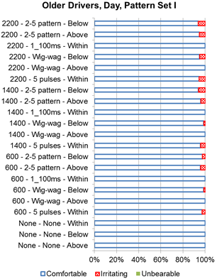
Figure 25. Graph. Older driver daytime discomfort rating for set I.

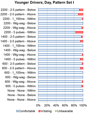
Figure 26. Graph. Younger driver daytime discomfort rating for set I.

During nighttime, more participants considered the LEDs to be unbearable, as illustrated in figure 27 and figure 28 for set I and figure 29 and figure 30 for set II. Trends in the data show that a larger proportion of the participants felt the flash patterns with the higher intensities were irritating or unbearable. Within set I, the wig-wag pattern with a target intensity of 2,200 candelas had the lowest number of participants, indicating it was comfortable for both older and younger drivers.

Reasons the participants gave an unbearable rating include the following:

• It was almost impossible to see the pedestrian.
  
  
• There was too much glare.
  
  
• Lights were too distracting.

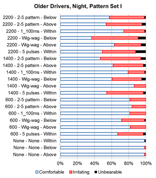
Figure 27. Graph. Older driver nighttime discomfort rating for set I.

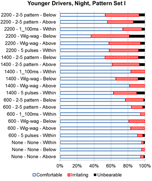
Figure 28. Graph. Younger driver nighttime discomfort rating for set I.

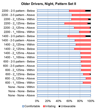
Figure 29. Graph. Older driver nighttime discomfort rating for set II.

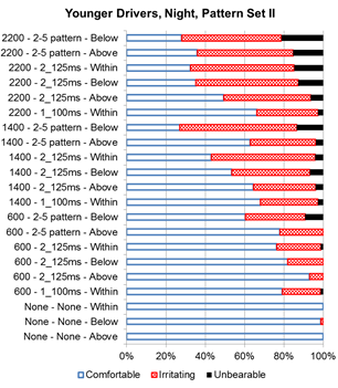
Figure 30. Graph. Younger driver nighttime discomfort rating for set II.

Concluding Survey

Queries 1 and 2—Driver Responses

The initial two queries asked the participants to indicate how the driver in the video would react to the pedestrian attempting to cross at the crosswalk. Table 18 highlights the number of participants who selected each of the potential responses for both queries 1 and 2 with the percent of participants shown in parentheses. Figure 31 shows a plot of the findings. For all of the devices studied, the answer selected by the majority of the participants was "stop." For two devices—the wig-wag pattern on the LEDs located below the sign and the sign without any active LEDs—had about one-third of the participants selecting the "confirm pedestrian is not crossing" answer while less than 17 percent selected that answer for the other two devices tested. Stated in another manner, the 2-5 below and the 100 ms within had more correct responses ("slow" or "stop" and "allow the pedestrian to cross") than the sign without LEDs or the sign with the LEDs below in a wig-wag pattern. The multiple flashes within a short time period, as is present with the 2-5 pattern, may be better at communicating the need to stop for a yellow device.

Table 18. Results for survey queries 1 and 2.

Flash Pattern	Number of Participants (Percent of Participants)
	Slowa	Stopb	Confirmc	Continued	Total
Within; 100	7 (22)	20 (63)	5 (16)	0 (0)	32 (100)
Below; wig-wag	3 (9)	18 (56)	11 (34)	0 (0)	32 (100)
Below; 2-5	5 (15)	23 (67)	6 (17)	0 (0)	34 (100)
Sign	23 (23)	44 (45)	29 (30)	2 (2)	98 (100)

^aI would slow and allow the pedestrian to cross the roadway.
^bI would stop and allow the pedestrian to cross the roadway.
^cI would confirm the pedestrian is not crossing before proceeding.
^dI would continue driving at the same speed.
Note: Flash patterns are defined as follows: 100 = one 100-ms flash pattern; wig-wag = wig-wag flash pattern; 2-5 = 2-5 flash pattern; and sign = no active LEDs.

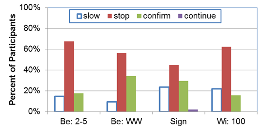
Figure 31. Graph. Results for survey queries 1 and 2.

Queries 3 and 4—Flash Pattern and LED Location

Queries 3 and 4 explored whether certain flash patterns and LED locations affected the participants' sense of urgency in needing to yield to a pedestrian. Each participant saw two pairs of videos. The results for queries 3 and 4 were combined for this review along with whether the sign was shown on the left side or the right side of the screen. To facilitate review of the results, findings were repeated for each pair combination (e.g., the results were shown for both the comparison of the within LEDs being on for 100 ms to sign (i.e., no active beacons) as well as sign (i.e., no active beacons) to within LEDs being on for 100 ms). Table 19 and table 20 show the results.

Table 19 contains the comparisons between having a sign with no active LEDs and the other combinations. For all of these comparisons, the majority of the participants selected the device with an active LED as communicating more urgency for yielding. For the comparison between sign and either below LEDs with a 2-5 flash pattern or below LEDs with four 25-ms flashes and one 100-ms flash, all of the participants felt the flashing device communicated a greater urgency to yield than the sign without an active LED. A majority of the participants (60 percent) felt the within LEDs with two 125-ms flashes communicated a greater urgency; however, 30 percent felt that neither device communicated urgency.

Table 19 also shows the results for the comparisons with the devices when the LEDs below the sign were active. When the 2-5 flash pattern was used with the LEDs below the sign, the participants felt it communicated a greater urgency as compared to the three patterns tested with the LEDs within the sign. The 2-5 pattern below the sign was favored by 90 percent of participants compared to the single 100-ms flash within the sign, by 78 percent compared to two 125-ms flashes within the sign, and 78 percent compared to four 25-ms flashes and one 200-ms flash within the sign. The comparison of the 2-5 flash pattern to the flash pattern with four 25-ms flashes and one 200-ms flash used with the below LEDs showed that the majority of the participants felt both devices communicated similar urgency (66 percent). The flash pattern for the below LEDs with four 25-ms flashes and one 200-ms flash was a subset of the below 2-5 flash pattern in that it was the "5" portion of the 2-5 pattern. Perhaps it was the multiple pulses that helped to communicate the urgency. The comparison of the 2-5 flash pattern with the pattern that only had the two pulses (below LEDs with two 125-ms flashes) had fewer participants feeling that both of these devices communicated a similar urgency (only 33 percent). This result provides some support that the multiple pulses helped to communicate urgency. A total of 22 percent of the participants felt the below LEDs with two 125-ms flashes communicated greater urgency as compared to the below 2-5 flash pattern, which added caution to the observation that more flashes were associated with greater urgency. The location of the LEDs may be another factor.

The comparison of the same number of flashes being used at different LEDs locations shows that participants believed the LEDs below the sign demonstrated more urgency than LEDs within the sign. For example, when two 125-ms pulses were used, the participants felt the LEDs below communicated a greater urgency (70 percent). The results for the four 25-ms flashes andone 200-ms flash also revealed that more participants felt the LEDs below (78 percent) showed greater urgency.

Within the comparisons of different flash patterns used with the within LEDs (see table 20), almost all of the participants (80 percent) felt the two-pulse pattern (i.e., two 125-ms pulses) and the five-pulse pattern (i.e., four 25-ms pulses and one 200-ms pulse) communicated the same urgency. The participants indicated that the two-pulse pattern (56 percent) communicated greater urgency over the one-pulse pattern (i.e., within LEDs with one 100-ms flash), or they felt those two patterns communicated a similar urgency (33 percent).

Table 19. Percent of participants who felt a sense of urgency to yield for signs with no active LEDs and LEDs below the sign.

Device 1	Device 2	Device 1 More Urgent (Percent)	Device 2 More Urgent (Percent)	Similar Urgency Both Devices (Percent)	Neither Device Conveys Urgency (Percent)
Sign	Within; 100	11	56	22	11
Sign	Within; 125(2)	0	60	10	30
Sign	Within; 25(4)+200	11	56	33	0
Sign	Below; 2-5	0	100	0	0
Sign	Below; 125(2)	0	89	11	0
Sign	Below; 25(4)+200	0	100	0	0
Below; 2-5	Within; one 100	90	0	0	10
Below; 2-5	Within; 125(2)	78	0	22	0
Below; 2-5	Within; 25(4)+200	78	0	11	11
Below; 2-5	Below; 125(2)	44	22	33	0
Below; 2-5	Below; 25(4)+200	25	13	63	0
Below; 2-5	Sign	100	0	0	0
Below; 125(2)	Within; one 100	89	0	11	0
Below; 125(2)	Within; 125(2)	70	0	30	0
Below; 125(2)	Within; 25(4)+200	90	0	10	0
Below; 125(2)	Below; 2-5	22	44	33	0
Below; 125(2)	Below; 25(4)+200	20	40	40	0
Below; 125(2)	Sign	89	0	11	0
Below; 25(4)+200	Within; one 100	82	0	18	0
Below; 25(4)+200	Within; 125(2)	89	0	11	0
Below; 25(4)+200	Within; 25(4)+200	78	0	11	11
Below; 25(4)+200	Below; 2-5	13	25	63	0
Below; 25(4)+200	Below; 125(2)	40	20	40	0
Below; 25(4)+200	Sign	100	0	0	0

Note: Flash patterns are defined as follows: 100 = one 100-ms flash pattern; 125(2) = two 125-ms flashes; 25(4)+200 = four 25-ms flashes and one 200-ms flash; 2-5 = 2-5 flash pattern; and sign = no active LEDs.

Table 20. Percent of participant results for sense of urgency to yield for LEDs above the sign.

Device 1	Device 2	Device 1 More Urgent (Percent)	Device 2 More Urgent (Percent)	Similar Urgency Both Devices (Percent)	Neither Device Conveys Urgency (Percent)
Within; 100	Within; 125(2)	11	56	33	0
Within; 100	Within; 25(4)+200	0	22	78	0
Within; 100	Below; 2-5	0	90	0	10
Within; 100	Below; 125(2)	0	89	11	0
Within; 100	Below; 25(4)+200	0	82	18	0
Within; 100	Sign	56	11	22	11
Within; 125(2)	Within; 100	56	11	33	0
Within; 125(2)	Within; 25(4)+200	10	0	80	10
Within; 125(2)	Below; 2-5	0	78	22	0
Within; 125(2)	Below; 125(2)	0	70	30	0
Within; 125(2)	Below; 25(4)+200	0	89	11	0
Within; 125(2)	Sign	60	0	10	30
Within; 25(4)+200	Within; 100	22	0	78	0
Within; 25(4)+200	Within; 125(2)	0	10	80	10
Within; 25(4)+200	Below; 2-5	0	78	11	11
Within; 25(4)+200	Below; 125(2)	0	90	10	0
Within; 25(4)+200	Below; 25(4)+200	0	78	11	11
Within; 25(4)+200	Sign	56	11	33	0

Note: Flash patterns are defined as follows: 100 = one 100-ms flash pattern; 125(2) = two 125-ms flashes; 25(4)+200 = four 25-ms flashes and one 200-ms flash; 2-5 = 2-5 flash pattern; and sign = no active LEDs.

Queries 5 and 6—Number of Pulses

For queries 5 and 6, the participants were asked to indicate how many flashes they could see on the left side and the right side of an active light bar. The research team used the term "flashes" rather than "pulses" because it has more common usage for the participants. The correct term would be pulses because "A flash is a light pulse or a train of light pulses, where a dark interval of at least 160 ms separates the light pulse or the last pulse of the train of light pulses from the next pulse or the first pulse of the next train of light pulses." ⁽¹⁵⁾(pg. 4)

The 2-5 flash pattern was used and had five pulses on the left side of the light bar and two pulses on the right side of the light bar. The frequency and percent of the responses by number of pulses is listed in table 21. One participant said there were eight flashes on each side. The researcher who worked with that participant believed the participant was counting the number of unique LEDs within the beacon rather than counting the number of pulses.

The majority of the participants (77 percent) correctly counted two pulses. A few of the participants (four) correctly counted five pulses. The majority of the participants (55 percent) saw three pulses when five pulses were present.

Table 21. Number of pulses on light bar.

Number of Pulses	Response for Side with Five Pulses		Response for Side with Two Pulses
	Frequency	Percent	Frequency	Percent
1	3	3	4	4
2	23	23	75	77
3	54	55	12	12
4	11	11	5	5
5	4	4	0	0
6	2	2	1	1
7	0	0	0	0
8	1	1	1	1
Total	98	100	98	100

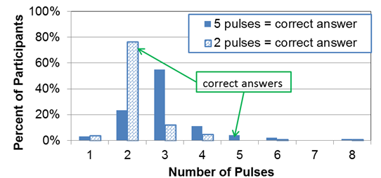
Figure 32. Graph. Number of pulses by percent of participants.

STATISTICAL ANALYSIS

The following subsections describe the statistical analyses performed on the data collected. It should be noted that when the term "significant" appears alone in these subsections, it indicates statistically significant (i.e., the differences found were unlikely to be a random variation but a systematic, measurable trend). Whenever appropriate, an explicit distinction is made to differentiate this term from "practical significance," which refers to the scale of a difference. For example, a difference may be found statistically significant in one of the analyses, but its magnitude could be such that is too small to be considered practically significant.

Pedestrian Detection Time

The data were initially split by daytime and nighttime conditions. Each set was analyzed using linear mixed effects models (LMMs). These kinds of models combine characteristics from both linear regression and analysis of variance (ANOVA). The model was specified such that appropriate accounts were given to the data structure, known associations between variables, and systematic variation in the response variable. The analysis treated the codependency of data points from the same drivers including a random effect for each participant in the experiment.

The analysis incorporated fixed effects for other variables of interest. In the case of detection time, the fixed effect variables were age, intensity, flash pattern, pedestrian height, and pedestrian position. Estimates, confidence intervals, and conclusions were later extracted for these effects. Due to the heavy skewness of the data, the analysis was performed over the natural logarithm of the detection time (see figure 33).

Figure 33. Equation. Natural logarithm of detection time.

Where:
ln(Detection_Time_i) = Natural logarithm of detection time for experiment i.
X_i = Vector of variable levels for experiment i.
β = Vector of coefficients for all variables in experiment (fixed effects, estimated).
α_j= Random effect for participant j (estimated).
ε_ij= Residual error for experiment i and subject j.

This statistical specification with a logged response allowed researchers to make inferences about the median detection time instead of the mean detection time. Because a logarithm transformation affects the distribution of the residual errors, the transformed mean is not equal to the original mean. However, an analysis on the transformed mean is equivalent to analyzing the median of the original scale (i.e., detection time) as long as normality or near-normality is achieved after the transformation. This is so because the normal distribution is symmetrical and also because the quartile distribution of the data is not affected by the log transformation. Therefore, each coefficient in the vector β can be interpreted (after exponentiation) as a multiplicative change on the median detection time per unit of explanatory variable.

All statistical analyses were performed using open-source statistical software. (See references 42-45.)

Daytime Time to Detect Pedestrian Direction

Table 22 shows the ANOVA on the variables in this analysis. These results indicate that target intensity had an impact on the detection time after accounting for the rest of variables in the table. In fact, except for two variables (LED location and lane) all of the experimental factors had a significant impact on detection time. The variables used in the following tables are defined as follows:

• Target intensity: Intensity of LEDs (0, 600, 1,400, or 2,200 candelas).
  
  
• Flash pattern: LED flash pattern (none, 2-5 flash pattern, wig-wag, one 100-ms flash, or five pulses).
  
  
• LED location: Location of LEDs in the assembly (above sign, below sign, or within sign).
  
  
• Pedestrian height: Height of the pedestrian when present (tall or short).
  
  
• Pedestrian position: Pedestrian position on crosswalk, when present (center, left, or right).
  
  
• Lane: Lane of vehicle with participant (left or right).
  
  
• Age: Age of participant (ranging from 19 to 85 years old).

Table 22. Daytime ANOVA for detection time fixed effects.

Variable	Numerator Degrees of Freedom (DF)	Denominator DF	F-value	p-value
Reference	1	2956	10730.10	< 0.0001
Target intensity	1	2956	22.44	< 0.0001
Flash pattern	4	2956	4.74	0.0008
LED location	2	2956	0.85	0.4270
Pedestrian height	1	2956	19.59	< 0.0001
Pedestrian position	3	2956	95.61	< 0.0001
Lane	1	28	2.11	0.1571
Age	1	28	7.37	0.0112

The coefficient estimates for daytime are shown in table 23. The comparison of flash patterns shows that 2-5 flash pattern produced longer detection times, though the p-values should be adjusted for multiple comparisons. The reference levels used for the base model in this study were no flash pattern, LED location is above, pedestrian height is tall, pedestrian position is none, and lane is left. The coefficient for target intensity in table 23 is small and statistically insignificant. The trend, however, is positive as is the trend at night (discussed in following subsection). Therefore, the no significance could be explained by the effect being smaller than the statistical power in the study. Indeed, examining the magnitude of the effect this coefficient implies, all other factors held equal (i.e. flash pattern, LED location in assembly, pedestrian height, pedestrian position, lane, and age of participant), the median response time increased by 0.00114 percent per additional candela of intensity (i.e., exp(0.0000114) = 1.0000114), which is about one-fourth of the magnitude of the same trend at night.

Table 23. Daytime detection time fixed effects coefficients.

Coefficient		Value	Standard Error	DF	t-value	p-value
Referencea		6.39000	0.21700	2956	29.5039	< 0.0001
Target intensity		0.00001	0.00001	2956	1.6846	0.0922
Flash pattern	2-5	0.05040	0.01800	2956	2.8054	0.0051 b
	100	0.04340	0.02380	2956	1.8231	0.0684 b
	Five flashes	0.04320	0.02380	2956	1.8135	0.0699 b
	Wig-wag	0.02260	0.01800	2956	1.2548	0.2097 b
LED location	Below	0.00686	0.01000	2956	0.6850	0.4934 b
	Within	-0.00422	0.02370	2956	-0.1783	0.8585 b
Pedestrian height—short		0.03850	0.00825	2956	4.6637	< 0.0001
Pedestrian position	Center	-0.22200	0.01320	2956	-16.8046	< 0.0001 b
	Left	-0.16700	0.01320	2956	-12.6137	< 0.0001 b
	Right	-0.16400	0.01330	2956	-12.3883	< 0.0001 b
Lane—right		0.17300	0.13400	28	1.2902	0.2075
Age		0.00947	0.00349	28	2.7139	0.0112

^aReference level used in model for each categorical variable base value: flash pattern = sign, LED location = above, pedestrian height = tall, pedestrian position = no pedestrian, and lane = left.
^bp-values for discrete factors with three or more levels need a multiple comparison adjustment.
Note: Flash patterns are defined as follows: 2-5 = 2-5 flash pattern; 100 = one 100-ms flash pattern; and wig-wag = wig-wag flash pattern.

The adjusted comparisons, shown in table 24, constitute evidence of the 2-5 flash pattern being the only flash pattern with statistically significantly longer detection times than no LEDs flashing during daytime conditions.

Table 24. Daytime simultaneous tests for general linear hypothesis of detection time flash pattern effects.

Condition 1	Condition 2	Estimatea	Standard Error	z-value	p-valueb	Significancec
2-5 flash pattern	None	0.05037	0.01796	2.805	0.0175	*
Wig-wag	None	0.02264	0.01805	1.254	0.5029
One 100-ms flash	None	0.04337	0.02379	1.823	0.1952
Five flashes	None	0.04323	0.02384	1.813	0.1986

^aEstimate is the difference between fixed effects coefficients corresponding to conditions 1 and 2.
^bAdjusted p-values were reported using a single-step method.
^cSignificance values are as follows: blank cell = p > 0.10; ~ = p < 0.10; * = p < 0.05; ** = p < 0.01; and *** = p < .0.001.

Each row in in table 24 represents a scientific hypothesis being tested statistically from the model results. For example, the first row of this table corresponds to the hypothesis that the natural logarithm of the average detection time under the 2-5 flash pattern is no different from the natural logarithm of the detection time when no flashing is present. The estimate for the difference of natural logarithm of detection time under each of these conditions is shown under the column titled "Estimate." The last four columns provide the basis for the assessment of the statistical significance of said difference in natural logarithm of detection time.

For the four intensity levels used in the study, table 25 shows that the magnitude of the intensity effect on median detection time is negligible during the daytime.

Table 25. Daytime magnitude of detection time intensity effect.

Target Intensity (Candela)	Estimated Increase in Median Detection Time (Percent)
0	0 (reference level)
600	0.7
1,400	1.6
2,200	2.4

There was a moderate impact of pedestrian height in detection time. Using the corresponding coefficient in table 23, results indicate that there was a 3.9 percent increase in detection time when using a short pedestrian cutout instead of a tall pedestrian cutout.

Nighttime Time to Detect Pedestrian Direction

Table 26 shows the ANOVA on the variables of interest. The results indicate that at night, all of the experimental factors had a significant impact on detection time except for lane.

Regarding flash patterns, the 2-5 flash pattern is again the pattern that triggered longer detection times. For nighttime, wig-wag was also associated with longer detection times.

Table 26. Nighttime ANOVA for detection time fixed effects.

Variable	Numerator DF	Denominator DF	F-value	p-value
Reference	1	6,016	39772.22	< 0.0001
Target intensity	1	6,016	85.61	< 0.0001
Flash pattern	5	6,016	30.74	< 0.0001
LED location	2	6,016	73.12	< 0.0001
Pedestrian height	1	6,016	22.06	< 0.0001
Pedestrian position	3	6,016	149.86	< 0.0001
Lane	1	60	1.46	0.2322
Age	1	60	8.74	0.0045

The coefficient estimates for nighttime are shown in table 27.

Table 27. Nighttime fixed effects coefficients for detection time.

Coefficient		Value	Standard Error	DF	t-value	p-value
Referencea		6.6900	0.1060	6,016	63.2133	0.0000
Target intensity		0.0000	0.0000	6,016	5.9727	0.0000
Flash pattern	2-5	0.0580	0.0154	6,016	3.7787	< 0.00b
	100	-0.0328	0.0184	6,016	-1.7841	0.0745b
	125(2)	-0.0077	0.0162	6,016	-0.4770	0.6330b
	Five pulses	-0.0172	0.0213	6,016	-0.8106	0.4180b
	Wig-wag	0.1280	0.0175	6,016	7.3196	< 0.001b
LED location	Below	0.1160	0.0091	6,016	12.7706	< 0.001b
	Within	0.0582	0.0139	6,016	4.1920	< 0.001b
Pedestrian height—short		0.0357	0.0075	6,016	4.7693	0.0000
Pedestrian position	Center	-0.1310	0.0118	6,016	-11.1563	< 0.001b
	Left	0.0490	0.0119	6,016	4.1094	< 0.001b
	Right	0.0465	0.0119	6,016	3.9206	< 0.001b
Lane—right		0.0950	0.0717	60	1.3252	0.1900
Age		0.0056	0.0019	60	2.9558	0.0045

^aReference level used in model for each categorical variable base value: flash pattern = sign, LED location = above, pedestrian height = tall, pedestrian position = no pedestrian, and lane = left.
^bp-values for discrete factors with three or more levels need a multiple comparison adjustment.
Note: Flash patterns are defined as follows: 2-5 = 2-5 flash pattern; 100 = one 100-ms flash pattern; 125(2) = two 125-ms flashes; and wig-wag = wig-wag flash pattern.

Table 28 shows the differences among flash patterns with statistical significance adjusted for multiple comparisons.

Table 28. Nighttime simultaneous tests for general linear hypothesis of flash patterns on detection time.

Condition 1	Condition 2	Estimatea	Standard Error	z-value	p-valueb	Significancec
2-5 flash pattern	None	0.058007	0.015354	3.778	< 0.001	***
Wig-wag	None	0.12806	0.017492	7.321	< 0.001	***
One 100-ms flash	None	-0.03284	0.018403	-1.784	0.248
Two 125-ms flashes	None	-0.00776	0.016156	-0.48	0.983
Five pulses	None	-0.0172	0.021267	-0.809	0.871

^aEstimate is the difference between fixed effects coefficients corresponding to conditions 1 and 2.
^bAdjusted p-values were reported using a single-step method.
^cSignificance values are as follows: blank cell = p > 0.10; ~ = p < 0.10; * = p < 0.05; ** = p < 0.01; and *** = p < 0.001.

There was statistical evidence of the 2-5 flash pattern delaying detection. The magnitude of this delay was very similar to the daytime delay (6 percent increase in median detection time at night versus 5.2 percent at daytime). However, at night, there was also evidence that the wig-wag flash pattern also delayed pedestrian detection. This delay is a substantial increase in detection time. Other variables being equal, median detection time was 13.7 percent longer for the wig-wag pattern than the median detection time with no LEDs active (i.e., 13.7 percent=[exp(0.12806) -1.0] x 100 percent).

The coefficient for target intensity at night was highly significant as opposed to being insignificant during the daytime. This coefficient was also larger at night by a factor of about 3.7 compared to the daytime. It is estimated that the median response time increased by 0.00369 percent per additional candela of intensity (i.e., exp(0.0000369) = 1.0000369) after controlling for other experimental factors. Table 29 shows the magnitude of the estimated impact of LED intensity. These magnitudes were substantial increases in median detection time.

Table 29. Nighttime magnitude of intensity effect on detection time.

Target Intensity (Candela)	Estimated Increase in Median Detection Time (Percent)
0	0.0 (reference level)
600	2.2
1,400	5.3
2,200	8.5

There was a moderate impact of pedestrian height on detection time. Using the coefficient in table 27, results indicate that there was a 3.6 percent increase in detection time when using a short pedestrian cutout instead of a tall pedestrian cutout.

Table 30 shows the relative effects of LED location with statistical significance adjusted for simultaneous comparisons. The shortest nighttime detection times occurred when the LEDs were located above the sign. Using this position as a reference level, the median detection time was 6 percent longer when the LEDs were located within the sign and 12.3 percent longer when the LEDs were located below the sign as compared to above. Finally, a comparison between LEDs within the sign against LEDs below the sign indicated that the median detection time was 6 percent longer at LEDs below the sign. All three contrasts were statistically significant. Table 31 summarizes these findings.

Table 30. Nighttime simultaneous tests for effect of LED location on detection time.

Condition 1	Condition 2	Estimatea	Standard Error	z-value	p-valueb	Significancec
Below	Above	0.116373	0.009112	12.771	< 0.001	***
Within	Above	0.058172	0.013877	4.192	< 0.001	***
Below	Within	0.058202	0.013906	4.185	< 0.001	***

^aEstimate is the difference between fixed effects coefficients corresponding to conditions 1 and 2.
^bAdjusted p-values were reported using a single-step method.
^cSignificance values are as follows: blank cell = p > 0.10; ~ = p < 0.10; * = p < 0.05; ** = p < 0.01; and *** = p < 0.001.

Table 31. Nighttime magnitude of LED location effect on detection time.

LED Location	Estimated Increase in Median Detection Time (Percent)
Above	0.0 (reference level)
Within	6.0
Below	12.3

Key Findings Regarding Detection Time

For the analysis focusing on detection time, (i.e., the time it took participants to indicate the direction of the cutout pedestrian from the moment the occlusion glasses were cleared), results indicate the following:

• As expected, detection time was longer at night than during the day.
  
  
• The age of the participants had an impact on detection time, both during the day and at night. Detection time for younger participants was shorter than detection time for older participants. It is estimated that there was an increase of 1 percent in median detection time per year of age during the daytime. At night, age made less of a difference. The corresponding estimate for this effect was an increase of 0.5 percent in median detection time per year of age.
  
  
• Pedestrian height had a very similar impact on detection time during the day and at night. Detection time was longer when the pedestrian cutout was short rather than tall. Results indicate an increase in median detection time of 3.9 percent during the daytime and an increase of 3.6 percent at night for the short pedestrian cutout compared to a tall cutout.
  
  
• In the case of pedestrian position, trends were the same for daytime and nighttime: detection times were longer when the pedestrian cutout was located on either side of the crosswalk compared to when it was located at the center of the road.
  
  
• Flash pattern also had a significant impact on detection time, though most of the differences between the different flash patterns were not statistically significant. Only two flash patterns produced significantly longer detection times than the base level of no flash pattern: the 2-5 flash pattern (used above and below sign) used during the day and at night and the wig-wag pattern (used above and below sign) at night only. Compared to no active flash pattern, there was an increase in median detection time for the 2-5 flash pattern by 5.2 percent during the day and of 6 percent at night. The wig-wag pattern caused an increase in median detection time of 13.7 percent.

LED location had a significant impact at night but not during the day. At night, detection was fastest when the LEDs were above the signs after controlling for other factors. Compared to the above sign LED location, the median detection time increased by 6 percent when the LEDs were within the sign and increased by an additional 6 percent when the LEDs were below the sign for a total increase of 12.3 percent when the below location was compared to the above location.

Accuracy of Detecting Pedestrian Direction

Similar to the analysis of detection time, the data were split by daytime and nighttime conditions. In the detection time analysis, only data representing the correct responses by the participant were utilized. For the accuracy analysis; however, the dataset also included the instances when participants indicated the incorrect walking direction. This analysis used both subsets (i.e., correct and incorrect answers) to evaluate changes in the rate of correct to total answers due to the different variables considered in the experimental design.

The analysis of the resulting dataset was performed on the framework of generalized linear mixed effects models (GLMMs). Similarly to LMMs, these kinds of models combine characteristics from both generalized linear regression and analysis of deviance. The analysis treated the co-dependency of data points from the same drivers including a random effect for each participant in the experiment. In doing so, the model gave an appropriate account to the correlation structure in the data. The model also included a simultaneous parametric estimation for the variables of interest (i.e., as fixed effects).

Similar to the analysis of detection time, the fixed effect variables were age, intensity, flash pattern, pedestrian height, and pedestrian position. Estimates, confidence intervals, and conclusions were later extracted for these effects. The formal specification of the statistical model for accuracy analysis is shown in figure 34.

Figure 34. Equation. Accuracy analysis.

Where:

Logit = Logit transformation, such that Logit(x) = Ln[x/(1 - x)].
Accuracy_Rate_ij = Accuracy rate at experiment i for participant j.
X'_ik = Vector of k variables whose levels are set for experiment i.

Since each experiment was only recorded once per participant, the best estimator for the accuracy rate was a binary variable, Z, representing the outcome of 1 if the response was correct, 0 otherwise. This variable was utilized as the response in the analysis. To make this a statistical model, an assumption that Z was binomially distributed was made, as shown in figure 35.

Figure 35. Equation. Accuracy rate.

The accuracy rate in the equation shown in figure 30 was estimated in the model. The known parameter n is the number of valid data points for each experiment/participant combination, which equals 1 in this study. The experiment design was such that only one response was obtained per experiment/participant combination. The model is then as shown in figure 36.

Figure 36. Equation. Logit model.

Where:

X' = Vector of explanatory variables.
α = Random effect, estimated for each participant.

The variables β and α in the equation shown in figure 36 were estimated by maximum likelihood.

Model Interpretation

The statistical specification linked the logit of the accuracy rate to a linear combination of the factors in the experiment design. Because the logit transformation is the natural logarithm of the odds of correct responses, inferences about the impact of changing experimental factors X to the accuracy rate should be made as follows: a marginal change of one variable in the linear predictor represents a multiplicative change in the odds of participant j correctly identifying the pedestrian direction. For experimental factor X_i1, with two levels, A and B, the equation in figure 37 defines the odds ratio that corresponds to coefficient, β₁.

Figure 37. Equation. Odds ratio corresponding to levels A and B of factor X_i1.

Where:

= Odds of level A of factor x_i1.
= Odds of level B of factor x_i1.

The equation in figure 37 indicates that the odds ratio (i.e., the ratio of odds of correct answers at level A to odds of correct answers at level B) is the exponential of the difference between levels multiplied by the corresponding regression coefficient. All statistical analyses were performed using R, an open-source statistical software. (See references 42-45.)

Daytime Accuracy of Detecting Pedestrian Direction

Table 32 shows the proportion of deviance corresponding by each variable in the analysis (i.e., analogous to an ANOVA table). This table indicates that target intensity had little or no impact on accuracy after accounting for the rest of the variables in the experiment design. Similarly, flash pattern did not have any influence on the odds of correctly detecting the pedestrian cutout. In contrast, this table shows that pedestrian position and participant age were the only two variables that were influential to accuracy of pedestrian detection. Specific coefficient estimates for daytime are shown in table 33.

Table 32. Daytime analysis of deviance for accuracy fixed effects.

Variables	Numerator DF	Sum of Squares	Mean Squares	F-value	p-valuea
Target intensity	1	0.812	0.812	0.812	0.367
Flash pattern	4	5.266	1.316	1.316	0.261
LED location	2	1.370	0.685	0.685	0.504
Pedestrian height	1	1.934	1.934	1.934	0.164
Pedestrian position	3	10.004	3.335	3.335	0.019
Lane	1	1.230	1.230	1.230	0.267
Age	1	12.130	12.130	12.130	< 0.001

^aThe statistics in this table are based on maximum likelihood estimates convergence to normality by virtue of the law of large numbers. Therefore, p-values were obtained from the limit case when DF in the denominator tends to infinity.

In table 33, only two coefficients were statistically significant: age of the participants and the position of the cutout when it faced to the right. The coefficient for age indicates that there was an inverse relationship between age and accuracy, as was expected. Except for the variables explicitly depicted, the rates in figure 38 correspond to the reference levels listed in table 33. From figure 38, it is evident that accuracy at daytime was high in general, with about 3 percent reduction in accuracy rates for the oldest participants when compared to the youngest participants in the study.

For the second statistically significant variable (i.e., pedestrian position to the right), the three p-values in table 33 should be adjusted for multiple comparisons. Table 34 shows multiple comparisons of interest and corresponding adjusted p-values. Although the trends are similar when comparing left and right sides with the center position, only the comparison between right side and center positions offers suggestive evidence of a real difference.

Table 33. Daytime accuracy fixed effects coefficients.

Daytime Coefficients		Value	Standard Error	z-value	p-value
Referencea		9.5480	1.3160	7.258	< 0.001
Target intensity		0.0004	0.0002	1.640	0.101
Flash pattern	2-5	-0.5800	0.6180	-0.938	0.34b
	100	-1.2440	1.1540	-1.079	0.281b
	Five flashes	-0.2500	1.2490	-0.200	0.841b
	Wig-wag	-0.9990	0.6120	-1.631	0.103b
LED location	Below	-0.3600	0.3320	-1.085	0.278b
	Within	0.2380	1.1790	0.202	0.840b
Pedestrian height—short		-0.4350	0.2990	-1.453	0.146
Pedestrian position	Center	-0.8780	0.8170	-1.075	0.282b
	Left	-1.5140	0.7840	-1.931	0.054b
	Right	-1.8500	0.7730	-2.391	0.017b
Lane—right		-0.3470	0.4520	-0.768	0.442
Age		-0.0490	0.0140	-3.483	< 0.001

^aReference level used in model for each categorical variable base value: flash pattern = sign, LED location = above, pedestrian height = tall, pedestrian position = no pedestrian, and lane = left.
^bp-values for discrete factors with three or more levels need a multiple comparison adjustment.
Note: Flash patterns are defined as follows: 2-5 = 2-5 flash pattern; 100 = one 100-ms flash pattern; and wig-wag = wig-wag flash pattern.

Table 34. Daytime simultaneous tests for general linear hypothesis of flash pattern accuracy effects.

Condition 1	Condition 2	Estimatea	Standard Error	z-value	Pr (> |z|)b	Significancec	Odds Ratio
Center	No pedestrian	-0.878	0.817	-1.075	0.6516		0.416
Left Side	Center	-0.636	0.419	-1.520	0.3660		0.529
Right Side	Center	-0.972	0.399	-2.438	0.0534	~	0.378
Both Sides	Center	-0.804	0.3735	-2.153	0.1073		0.448
Left Side	Right Side	0.3355	0.3324	1.009	0.6948		1.399

^aEstimate is the difference between fixed effects coefficients corresponding to conditions 1 and 2.
^bAdjusted p-values were reported using a single-step method.
^cSignificance values are as follows: blank cell = p > 0.10; ~ = p < 0.10; * = p < 0.05; ** = p < 0.01; and *** = p < 0.001.

Figure 38 and figure 39 show accuracy rates by pedestrian cutout position and age after accounting for other experimental factors. The extreme difference in accuracy curves when the pedestrian cutout is present is between the center and right-side positions as shown in figure 39. This difference was negligible for younger drivers and was a modest 3 percent for older drivers.

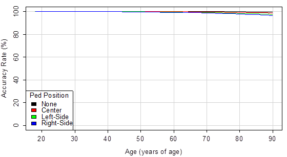
Figure 38. Graph. Daytime estimated accuracy rate by age and pedestrian position.

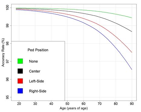
Figure 39. Graph. Close-up view of daytime estimated accuracy rate by age and pedestrian position.

Nighttime Accuracy of Detecting Pedestrian Direction

Table 35 shows the analysis of deviance of the model in this analysis. These results indicate that at night, all the experimental factors have a significant impact on the accuracy rate, except for lane. The coefficient estimates for nighttime are shown in table 36.

Table 35. Nighttime analysis of deviance for accuracy fixed effects.

Variables	Numerator DF	Sum of Squares	Mean Squares	F-value	p-valuea
Target intensity	1	14.174	14.174	14.174	< 0.001
Flash pattern	5	13.470	2.694	2.694	0.019
LED location	2	50.289	25.145	25.145	< 0.001
Pedestrian height	1	15.686	15.686	15.686	< 0.001
Pedestrian position	3	95.724	31.908	31.908	< 0.001
Lane	1	1.363	1.363	1.363	0.243
Age	1	11.166	11.166	11.166	< 0.001

^aThe statistical quantifiers in this table are based on maximum likelihood estimates convergence to normality by virtue of the law of large numbers. Therefore, p-values were calculated in the limit when DF in the denominator tended to infinity.

Table 36. Nighttime accuracy fixed effects coefficients.

Nighttime Coefficients		Value	Standard Error	t-value	p-value
Referencea		8.2800	0.6580	12.575	< 0.0001
Target intensity		-0.0003	0.0001	-2.789	0.0053
Flash pattern	2-5	-0.2810	0.2440	-1.149	0.2506b
	100	0.3250	0.3020	1.073	0.2831b
	125(2)	0.2070	0.2590	0.802	0.4223b
	Five flashes	0.1160	0.3430	0.338	0.7357b
	Wig-wag	-0.4010	0.2750	-1.458	0.1447b
LED location	Below	-1.0900	0.1410	-7.762	< 0.0001b
	Within	-0.7780	0.2320	-3.349	0.0008b
Pedestrian height—short		-0.4540	0.1160	-3.918	0.0001
Pedestrian position	Center	-1.8900	0.4090	-4.625	< 0.0001b
	Left	-2.9200	0.4000	-7.305	0.0000b
	Right	-2.8400	0.4010	-7.101	0.0000b
Lane—right		0.3300	0.3200	1.031	0.3025
Age		-0.0283	0.0085	-3.342	0.0008

^aReference level used in model for each categorical variable base value: flash pattern = sign, LED location = above, pedestrian height = tall, pedestrian position = no pedestrian, and lane = left.
^bp-values for discrete factors with three or more levels need a multiple comparison adjustment.
Note: Flash patterns are defined as follows: 2-5 = 2-5 flash pattern; 100 = one 100-ms flash pattern; 125(2) = two 125-ms flashes; and wig-wag = wig-wag flash pattern.

There was no evidence of a difference in accuracy of answers due to different flash patterns after accounting for other relevant factors. Compared to the no flash pattern, only the 2-5 and wig-wag flash patterns seemed to have hindered accuracy (i.e., negative coefficients), but the data did not offer statistical evidence that these differences in fact diverged from zero. However, it is interesting that these two flash patterns were the same for which the analysis of detection time found evidence of being counterproductive.

Also, similar to the results of the detection time analysis, the accuracy analysis found that intensity of the LEDs had an adverse effect. Using the base conditions from table 36, figure 40 and figure 41 demonstrate in absolute terms the impact of target intensity across the range of ages of participants. Also shown in figure 41 is the significant impact of participant age in accuracy of detection. Table 37 shows the odds ratios for the four intensity levels in this study. This table demonstrates that the odds of correct detections fell with increasing intensity.

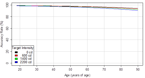
Figure 40. Graph. Nighttime estimated accuracy rate by age and LED intensity.

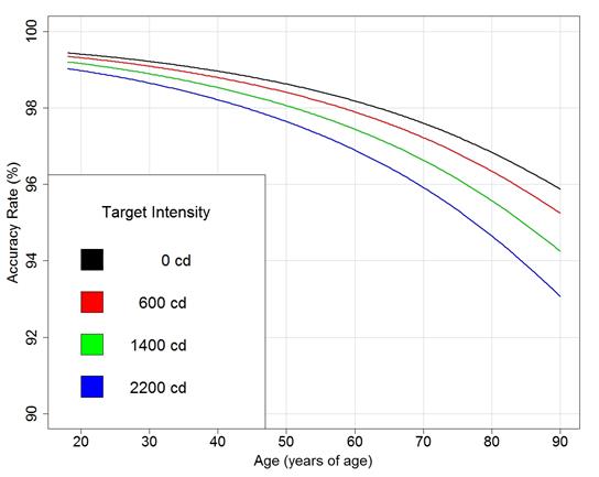
Figure 41. Graph. Close-up view of nighttime estimated accuracy rate by age and LED intensity.

Table 37. Nighttime odds ratio of correct detection intensity levels.

Target Intensity (Candela)	Odds Ratio (Correct Detections)
0	1.00 (reference level)
600	0.86
1,400	0.71
2,200	0.58

Table 38 shows the relative effects of pedestrian location with statistical significance adjusted for simultaneous comparisons. Compared to pedestrian in the center of the crosswalk, placing the pedestrian on either side caused a significant drop in the odds of accurate answers. The difference between left and right sides was found to be not significant.

Table 38. Nighttime simultaneous linear hypotheses for pedestrian position effect on accuracy.

Condition 1	Condition 2	Estimatea	Standard Error	z-value	Pr( >|z|)b	Significancec	Odds Ratio
Center	No pedestrian	-1.88952	0.40859	-4.625	< 0.001	***	0.151
Left side	Center	-1.03111	0.15249	-6.762	< 0.001	***	0.357
Right side	Center	-0.95434	0.15456	-6.175	< 0.001	***	0.385
Both sides	Center	-0.99272	0.13994	-7.094	< 0.001	***	0.371
Left side	Right side	-0.07677	0.12629	-0.608	0.914		0.926

^aEstimate is the difference between fixed effects coefficients corresponding to conditions 1 and 2.
^bAdjusted p-values were reported using a single-step method.
^cSignificance values are as follows: blank cell = p > 0.10; ~ = p < 0.10; * = p < 0.05; ** = p < 0.01; and *** = p < 0.001.

Table 39 shows the relative effects of LED location with statistical significance adjusted for simultaneous comparisons. The most accurate detections at night occurred, as well as the shortest detection times, when the LEDs were located above the sign. Other variables kept equal, the odds of accurate detection with LEDs below the sign were about one-third of the odds with LEDs above sign. The data did not provide evidence supporting any significant difference in odds of accurate detection when comparing LEDs located below and within the sign.

Table 39. Nighttime simultaneous linear hypotheses on LED location effect on accuracy.

Condition 1	Condition 2	Estimatea	Standard Error	z-value	Pr( >|z|)b	Significancec	Odds Ratio
Below	Above	-1.0943	0.141	-7.762	< 0.001	***	0.335
Within	Above	-0.7783	0.2324	-3.349	0.00206		0.459
Below	Within	-0.316	0.2161	-1.462	0.30099		0.729

^aEstimate is the difference between fixed effects coefficients corresponding to conditions 1 and 2.
^bAdjusted p-values were reported using a single-step method.
^cSignificance values are as follows: blank cell = p > 0.10; ~ = p < 0.10; * = p < 0.05; ** = p < 0.01; and *** = p < 0.001.

Key Findings Regarding Accuracy of Detection

For the analysis focusing on accuracy of detection, results indicate the following:

• As expected, detection accuracy was higher during the daytime than at night.
  
  
• The age of participants had an impact on accuracy, both during the daytime and at night. Accuracy at daytime was high in general. The analysis indicated, however, a measurable but small reduction in accuracy by age. For example, it was estimated that there was a difference of about 3 percent in accuracy rate between the oldest participants (85 years old) and the youngest participants (19 years old) when they were presented with no flashing LEDs and the tall pedestrian was placed at either the right or the left side. Similarly, the age of the participant had a significantly larger effect under nighttime conditions compared to daytime conditions. For the same scenario described (i.e., no LED and the tall pedestrian cutout positioned at either the right or the left side of the crosswalk) the difference between accuracy rates of a participant 85 years old and another participant 19 years old was estimated at about 8 percent.
  
  
• Regarding pedestrian height, accuracy was higher when the pedestrian cutout was tall compared to when it was short.
  
  
• Pedestrian position had an impact on accuracy. The evidence for this effect was strong at night but only suggestive during the daytime. In general, locating the pedestrian at the center of the crosswalk had more accurate responses compared to when the cutout was located at either side of the crosswalk. In particular for daytime, only the difference between right-side and center position had a statistical significance, and it was minimal. For nighttime, however, the trends were the same, but the data provided convincing evidence of an impact of pedestrian position: lower accuracy could be attributed to placing the pedestrian cutout on either side of the crosswalk (i.e., closer to the LED assembly) compared to the center position. This finding suggests that being further away from the active LEDs makes accurately detecting pedestrian walking direction easier. As with daytime, no statistical difference was found between the left and right sides at night.
  
  
• No evidence was found of the flash pattern having a significant impact on accuracy during the day and at night.
  
  
• LED location had a significant impact on accuracy at night but not during the day. At night, detection was most accurate when the LEDs were above the signs after controlling for other factors. Placing the LEDs within the sign led to slightly better accuracy rates than the below location, which was similar to the trends observed for detection time across LED locations. However, this small difference in accuracy rates was not found statistically significant.

Discomfort Glare

The discomfort data obtained from participants' responses were categorized by daytime and nighttime conditions for the analysis. Similar to the analysis of detection times, the only discomfort data used in the analysis were those provided after a correct response was given on pedestrian direction. The discomfort analysis statistically evaluated the changes in the expressed discomfort that could be attributed to the different variables considered in the experimental design.

The analysis used GLMMs to account for repeated measures taken from the same participants. Similar to the previous two analyses, variables age, intensity, flash pattern, pedestrian height, and pedestrian position were coded as fixed effects, with their corresponding standard errors and confidence intervals. Random intercepts per participant were included as a random effect to induce the correlation expected between all responses from each participant.

The discomfort level expressed by the participants could be described as a discrete partition of a continuous non-observable variable that indicated true discomfort. In other words, the true discomfort experienced was ideally a continuous, monotonic function. The goal of the analysis was, in essence, to characterize the relationship between the unobserved real discomfort and the three-level, discrete variable corresponding to the question asked to participants after each experiment (where the only possible answers were comfortable, irritating, and unbearable). The relationship between the true and discrete discomfort variables can be idealized by the plot shown in figure 42 for a given level of an experimental factor:

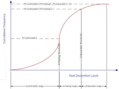
Figure 42. Graph. Idealized relationship between discrete and real discomfort scales.

It can be logically concluded from this graph that the cumulative frequency of answers from all participants defines incremental thresholds in the real discomfort level. Therefore, the statistical analysis quantified how the thresholds changed in response to the variability of the factors in the experiment design. These changes should directly correspond to changes in the idealized continuous discomfort scale.

Given that the odds corresponding to the cumulative frequency at any of the two thresholds are proportional to the odds corresponding to the cumulative frequency at the other threshold, then any of these cumulative frequencies can be related to the explanatory factors, as shown in figure 43.

Figure 43. Equation. Cumulative frequency.

Where:

Cumulative_frequency_dij = Cumulative frequency of answers below threshold d in the discretized scale of discomfort at experiment i for participant j.
θ_d= Log-odds of the threshold for discomfort level d at base conditions (estimated).

Model Interpretation

The statistical specification linked the logit of the cumulative rate in the discomfort scale to a linear combination of the factors in the experiment design. Because the logit transformation is the natural logarithm of the odds, inferences about the impact of changing experimental factors X to the discomfort rate cannot be made in a linear fashion. Instead, inferences should be made similar to interpreting a logistic model as follows: for a given threshold d, a positive marginal change of one variable in the linear predictor represents a multiplicative increase in the odds of the participant indicating any higher level of discomfort compared to the odds of any lower level of discomfort. In other words, for a given threshold d, a positive coefficient indicates an increase in the odds of indicating any higher level of discomfort at that threshold. Similarly, a negative coefficient indicates a decrease in the odds of any higher level of discomfort at that threshold.

For experimental factor X_i1 with two levels, A and B, the equation is shown in figure 44.

Figure 44. Equation. Odds ratio for levels A and B of variable X_i1 at a maximum level of discomfort.

The quantities in parenthesis shown in figure 44 are odds ratios (i.e., the ratio of odds of level of discomfort d or below at X_i1 = A to odds of level of discomfort d or below at X_i1 = B). This relationship implies that the odds ratio at both thresholds should be proportionally related to changes in all factors in the experimental design. Such condition is a critical assumption of the model. Re-expressing the last equality yields an equivalent form that can be used to verify the proportional odds assumption of the model, as shown in figure 45.

Figure 45. Equation. Revised odds ratio.

The researchers verified that this equality reasonably held for various marginal odds obtained from partitioning the data by levels of the variables of interest (i.e., intensity and flash pattern) as well as by the age of participants. Therefore, the researchers found this model specification appropriate for analyzing the discomfort response. All statistical analyses were performed using R, an open-source statistical software. (See references 42-46.)

Daytime Discomfort

As an alternative to an analysis of deviance, Table 40 shows the likelihood ratio tests for models that incrementally add each experimental variable in the analysis.

Table 40. Daytime likelihood ratio tests for incremental discomfort fixed effects.

Variable	DF	Log Likelihood	Chi-Squared Statistic	p-valuea
Reference	N/A	-248.5	N/A	N/A
Target intensity	1	-230.96	35.0783	< 0.001
Flash pattern	4	-193.54	74.8384	< 0.001
LED location	2	-193.5	0.0775	0.96198
Pedestrian height	1	-192.82	1.3694	0.24192
Pedestrian position	3	-189.57	6.5003	0.08965
Lane	1	-189.54	0.0463	0.82961
Age	1	-189.53	0.0165	0.89784

^aThe statistical quantifiers in this table were based on the expected convergence to normality of the log-likelihood function by virtue of the law of large numbers.
N/A = Not applicable.

Table 40 indicates that, after accounting for target intensity and flash pattern, little or no gains in explanatory power resulted from including additional variables. A notable exception in this table is the inclusion of pedestrian position; it showed a minor improvement that is barely statistically insignificant. However, the deviances should be taken as a preliminary assessment of the importance of variables in the analysis. To draw conclusions, specific coefficient estimates for a daytime model accounting for all variables simultaneously were obtained, as shown in table 41.

The only coefficient statistically significant in table 41 corresponds to LED target intensity. This is not surprising, given that the vast majority of discomfort answers during daytime were comfortable. This resulted in a problematic statistical estimation of the first two coefficients in the table (i.e., the discomfort thresholds). Even though the information about the thresholds of the discomfort scale is limited, there is strong evidence of the discomfort increasing with increasing intensity (per the target intensity coefficient in the table). All other factors held equal (i.e., flash pattern, LED location in assembly, pedestrian height, pedestrian position, lane, and age of participant), the odds of a higher level of discomfort increased by 0.089 percent per additional candela of intensity (i.e., (1 - exp(8.88E-04 ) × 100 percent = 0.089 percent). Table 42 shows the odds ratios for increase discomfort level at the four intensity values included in this research.

Table 41. Daytime discomfort fixed effect coefficients.

Coefficient		Value	Standard Error	z-value	p-value
Intercepta	First threshold (comfortable | irritating)	39.87	451.2	0.088	0.930
	Second threshold (irritating | unbearable)	44.83	451.21	0.099	0.921
Target intensity		0.0009	0.0002	3.9340	0.0004
Flash pattern	2-5	27.6000	452.0000	0.0610	0.951b
	100	25.7000	696.0000	0.0370	0.971b
	Five flashes	29.7000	696.0000	0.0430	0.966b
	Wig-wag	25.7000	452.0000	0.0570	0.955b
LED location	Below	-0.0721	0.3330	-0.2170	0.829b
	Within	-1.8200	298.0000	-0.0060	0.995b
Pedestrian height—short		0.3120	0.2860	1.0900	0.2760
Pedestrian position	Center	-0.4310	0.4740	-0.9090	0.364b
	Left	-0.1780	0.4570	-0.3890	0.697b
	Right	0.4820	0.4580	1.0510	0.293b
Lane—right		-0.5840	2.7500	-0.2120	0.8320
Age		-0.0093	0.0718	-0.1290	0.8980

^aReference level used in model for each categorical variable base value: flash pattern = sign, LED location = above, pedestrian height = tall, pedestrian position = no pedestrian, and lane = left.
^bp-values for discrete factors with three or more levels need a multiple comparison adjustment. Therefore, p-values in this table should not be used unless they correspond to a continuous variable or to a discrete factor of two levels.
Note: Flash patterns are defined as follows: 2-5 = 2-5 flash pattern; 100 = one 100-ms flash pattern; and wig-wag = wig-wag flash pattern.

Table 42. Daytime odds ratios for higher level of discomfort by target intensity level.

Target Intensity (Candela)	Odds Ratio
0	1.00 (reference level)
600	1.70
1,400	3.47
2,200	7.05

Nighttime Discomfort

Table 43 shows a preliminary assessment of the importance of experimental variables in the results based the deviance breakdown of the nighttime data. These results indicate that at night, all the experimental factors influenced the discomfort level.

Table 43. Nighttime likelihood ratio tests for incremental discomfort fixed effects.

Variable	DF	Log Likelihood	Chi-squared Statistic	p-valuea
Reference	N/A	-3699.1	N/A	N/A
Target intensity	1	-3272.5	853.2187	< 0.001
Flash pattern	5	-3145.2	254.7609	< 0.001
LED location	2	-3104.0	82.2763	< 0.001
Pedestrian height	1	-3101.6	4.7844	0.02872
Pedestrian position	3	-3045.6	112.1452	< 0.001
Lane	1	-3043.2	4.6482	0.03109
Age	1	-3035.3	15.8501	< 0.001

^aThe statistical quantifiers in this table were based on the expected convergence to normality of the log-likelihood function by virtue of the law of large numbers.
N/A = Not applicable.

The coefficient estimates for nighttime are shown in table 44, which can be used to draw formal conclusions about the variables influencing discomfort at night. Results indicate that all factors had a bearing in the discomfort level expressed by participants, except for the lane (right or left) where the participant parked.

Table 44. Nighttime discomfort fixed effect coefficients.

Coefficient		Value	Standard Error	z-value	p-value
Intercepta	First threshold (comfortable | irritating)	4.2135	0.4709	8.9470	< 0.001
	Second threshold (irritating | unbearable)	6.8120	0.4763	14.3030	< 0.001
Target intensity (candela)		0.0010	0.0001	18.8520	< 0.001
Flash pattern	2-5	2.5600	0.2640	9.7190	< 0.001b
	100	1.2800	0.2820	4.5300	< 0.001b
	125(2)	2.1700	0.2660	8.1470	< 0.001b
	Five flashes	2.0600	0.2930	7.0460	< 0.001b
	Wig-wag	2.2400	0.2750	8.1720	< 0.001b
LED location	Below	0.6200	0.0802	7.7340	< 0.001b
	Within	0.6440	0.1390	4.6260	< 0.001b
Pedestrian height—short		-0.1490	0.0666	-2.2370	0.0253
Pedestrian position	Center	-0.1230	0.1080	-1.1350	0.2564b
	Left	0.5290	0.1060	4.9870	< 0.001b
	Right	0.4420	0.1080	4.0920	< 0.001b
Lane—right		0.2500	0.2660	0.9400	0.3471
Age		-0.0153	0.0070	-2.1790	0.0293

^aReference level used in model for each categorical variable base value: flash pattern = sign, LED location = above, pedestrian height = tall, pedestrian position = no pedestrian, and lane = left.
^bp-values for discrete factors with three or more levels need a multiple comparison adjustment.
Note: Flash patterns are defined as follows: 2-5 = 2-5 flash pattern; 100 = one 100-ms flash pattern; 125(2) = two 125-ms flashes; and wig-wag = wig-wag flash pattern.

Target Intensity

Not surprisingly, target intensity of the LEDs had a positive relationship with nighttime discomfort level. After accounting for all other factors, this analysis indicates that the odds of higher discomfort increased by 0.102 percent per additional candela of intensity. Table 45 shows the odds ratios corresponding to the target intensities used in the study. Similarly, there was convincing evidence of a reduction in discomfort levels associated with placing the short pedestrian in the crosswalk compared to placing the tall pedestrian.

Table 45. Nighttime odds ratios of higher discomfort by target intensity level.

Target Intensity (Candela)	Odds Ratio
0	1.00 (reference level)
600	1.84
1,400	4.17
2,200	9.43

Flash Pattern

There was also strong evidence of an increase in discomfort under all different flash patterns compared to no LEDs flashing after accounting for other relevant factors. Positive coefficients indicate that the odds of higher discomfort were statistically higher than the base condition of no flash pattern. It was of interest; however, to evaluate simultaneous comparisons to determine if there was any particularly flash pattern associated with a high risk of discomfort scores. Due to the particular statistical specification of this analysis, the researchers carried the multiple comparisons by computing the multivariate Hotelling's T² statistic in contrast with the previous two analyses. This is a single measure of significance for a set of independent simultaneous hypotheses that involve the coefficient estimates and their corresponding covariance. Since there were six different flash patterns, this methodology allowed up to five simultaneous comparisons for this factor. The researchers defined three comparisons that address the question of interest, shown in table 46. The unique and small p-value for this table (1.676E-05) indicates that the test rejected the prospect that all hypotheses were true simultaneously. The last two columns in this table show the expected range of variation in odds ratio for each hypothesis in an overall 95 percent confidence region associated with the simultaneous comparisons. From these columns, the results indicate the following:

• The odds ratio between the group of all the flash patterns to no flash pattern at all was statistically different from 1. The odds of a higher discomfort level were significantly larger for the group of all flash patterns.
  
  
• The odds ratio for higher discomfort was not different from 1 when comparing the 2-5 or wig-wag flash patterns to the rest of flash patterns (not including none).
  
  
• The odds ratio for higher discomfort was not different from 1 when comparing the 2-5 flash pattern to the wig-wag flash pattern.

Table 46. Nighttime simultaneous hypotheses for flash pattern discomfort effect.

Hypothesis on Odds Ratios	Minimum Estimate of Odds Ratio	Maximum Estimate of Odds Ratio
(All flashing) ÷ (None) = 1	2.10	29.42
(2-5 or wig-wag) ÷ (All others flashing) = 1	0.91	3.41
(2-5) ÷ (wig-wag) = 1	0.79	2.40

For this table, a multivariate T² statistic was computed to test the three hypotheses simultaneously. The corresponding T² statistic was 108.07; this statistic follows the F-distribution with 16 DF in the numerator and 6,075 DF in the denominator. The corresponding F-statistic is then F(16; 6,075) = 6.738. Because the corresponding critical F-statistic for a 95 percent confidence of simultaneous comparisons is 1.645, the result of this statistical test indicates that there is convincing evidence that at least one hypothesis in table 46 is such that it the confidence interval does not contain 1.0. From this table, it is clear that such hypothesis is the one comparing all flashing patters to none.

LED Location

Table 47 shows the relative effects of LED location with statistical significance adjusted for simultaneous comparisons. The T² statistic corresponding to this table indicates convincing evidence of higher discomfort when the LEDs were located below the sign compared to when they were located above the sign. In contrast, there was no sufficient evidence that locating LEDs within the sign resulted in higher discomfort as compared to above the sign. For this table, the resulting T² statistic was 64.9134; the corresponding F-statistic from a F(16, 6,074) distribution was 4.047. The critical F-statistic for a 95 percent confidence of all simultaneous comparisons was 1.645, with a corresponding p-value of 9.033E-08 for a test on the two hypotheses simultaneously.

Table 47. Nighttime simultaneous hypotheses on LED location discomfort effect.

Hypothesis	Minimum Estimate of Odds Ratio	Maximum Estimate of Odds Ratio
(Below) ÷ (Above) = 1	1.23	2.81
(Within) ÷ (Above) = 1	0.93	3.89

Pedestrian Position

Table 48 shows the expected ranges for the relative effects of pedestrian position, given that they were compared simultaneously. There was convincing evidence of higher discomfort when the pedestrian was located at either side compared to when the pedestrian was located at the center of the crosswalk. In contrast, there was no sufficient evidence that having the pedestrian in the crosswalk resulted in higher discomfort compared to when no pedestrian was present. The T² statistic for this table was 73.225; the test statistic was F(16, 6,074) = 4.565. The critical F-statistic for a 95 percent confidence of all simultaneous comparisons was 1.645, with corresponding p-value of 3.353E-09.

Table 48. Nighttime tests for simultaneous hypotheses on discomfort effect of pedestrian location.

Hypothesis	Minimum Estimate for Odds Ratio	Maximum Estimate for Odds Ratio
(Pedestrian) ÷ (No pedestrian) = 1	0.81	2.16
(Either side) ÷ (Center) = 1	1.24	2.73
(Left side) ÷ (Right side) = 1	0.59	1.42

Age

Finally, this analysis found that driver age influenced the odds of higher discomfort after controlling for other factors in the experimental design. This decreasing discomfort trend is shown in figure 46 when no pedestrian was in the crosswalk and the LEDs were set at 2,200 candelas using the 2-5 flash pattern.

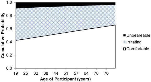
Figure 46. Graph. Estimated cumulative probabilities by age of participant for the discrete scale of discomfort when using 2,200 candelas of intensity and the 2-5 flash pattern.

Key Findings Regarding Discomfort of Detection

For the analysis focusing on discomfort, results indicate the following:

• There were clear differences in discomfort between daytime and nighttime. It was estimated that the odds of increasing discomfort were only influenced by LED intensity during the day, whereas almost all experimental factors had an impact at night.
  
  
• LED intensity had a significant impact on discomfort levels during the nighttime only.
  
  
• The age of participants had an impact on discomfort levels during the nighttime only. Discomfort tended to decrease with increasing participant age.
  
  
• Pedestrian position had an impact on discomfort level during the nighttime only. There was no evidence for increasing discomfort levels when the pedestrian was present compared to when the pedestrian was absent. However, locating the pedestrian at any side of the crosswalk yielded higher discomfort compared to when the pedestrian was located at the center of the crosswalk. This effect is probably associated with the proximity to the active LEDs. No evidence of higher discomfort was found when the pedestrian cutout was placed on the right side compared to when it was placed on the left side.
  
  
• For nighttime only, there was convincing evidence of the flash pattern having an impact on discomfort levels. Not surprisingly, this analysis found a significant increase of discomfort associated with any flash pattern compared to no flash pattern at all.
  
  
• For nighttime only, LED location had a significant impact on discomfort levels. This analysis found evidence of higher discomfort levels when the LEDs were located below the sign compared to LEDs above the signs after controlling for other factors. Although the trend is similar when comparing LEDs within the sign to LEDs above the sign, this analysis did not find this difference statistically significant.