U.S. Department of Transportation
Federal Highway Administration
1200 New Jersey Avenue, SE
Washington, DC 20590
202-366-4000
Federal Highway Administration Research and Technology
Coordinating, Developing, and Delivering Highway Transportation Innovations
 |
| This report is an archived publication and may contain dated technical, contact, and link information |
|
Publication Number: FHWA-RD-02-082 Date: August 2006 |
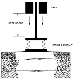
The FWD is an impulse loading device used to simulate moving wheel loads and measure the corresponding pavement response. The FWD applies a dynamic load by dropping a mass from a predetermined height, as illustrated in figure 61. The mass drops onto a foot plate connected to a rigid 30-cm diameter base plate by means of thick rubber buffers, which act as springs. The falling weight subassembly is furnished so that different load magnitudes can be applied by varying the mass and drop height. The FWD load signal is a transient pulse with a duration of 25 to 35 milliseconds. Seismic transducers, known as geophones, measure the resulting pavement deflection.
Figure 61. Falling Weight Deflectometer.
The FWD was specified in the contract to test the experimental pavement sections in Nevada, Delaware, California, and New Mexico in an effort to detect ASR. The treatment types, number of slabs per section, and section lengths were variable between the four test sites. Detailed information regarding treatments and test site layout is contained in the previous sections of this report. A brief summary of general cross section information for each site is shown in table 47.
| Site | Joint Spacing, ft | Mean Slab Thickness1, inches | Base Type | Base Thickness, inches | Shoulder Type |
|---|---|---|---|---|---|
| Nevada | 12-13-19-18 | 8.0 | CTB | 6.0 | PCC |
| Delaware | 40 | 8.0 | CTB | 6.0 | Curb and Gutter |
| California | 12-13-19-18 | 8.25 | CTB | 4.0 | AC |
| New Mexico | 18 | 8.8 | CTB | 6.0 | Curb and Gutter |
1 The actual slab thicknesses varied from section to section within each site.
1 m = 3.28 ft
1 inch = 2.54 cm
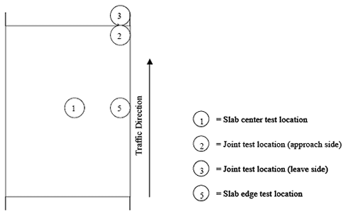
For each of the concrete slabs located at each test site, FWD testing was conducted at the center of slab, edge of slab, and in the right wheelpath at the joint. At each test point, at least one drop at each of three load levels—40.03, 53.38, and 71.17 kilonewtons (kN) (9, 12, and 16 kips)—was made. Figure 62 provides an illustration of the testing locations within each slab. Except where otherwise stated, the data was collected with the following sensor and load configuration for the slab center and joint tests:
Figure 62. Illustration of testing locations.
FWD testing was conducted on all sites in all 5 years of the performance monitoring period— 1994 through 1998. The testing was generally conducted between the months of October and December of each year. Weather-related problems (rain and snow) prevented the collection of FWD data other than the center slab deflections in the year 1996 for the California and Nevada sites.
Before analyzing any of the deflection data collected, the data were normalized to a 4,086-kg load to account for slight variations in the actual load applied by the FWD. This normalization process was done using standard linear extrapolation techniques and is a routine operation. Further, to make valid performance comparisons on a year-to-year basis, it was necessary to ensure that the testing was done at approximately the same locations within each site. This was an important step in establishing the analysis database. Comparisons of the raw FWD data from each year and each site were made to ensure that test points were indeed collected in the same location. In a few cases, additional test points were discovered in a given year that did not have corresponding test points in the other years. Such data was not considered in further analysis; however, the data was retained in the final deflection database.
The elastic modulus of the concrete, EPCC, and the joint deflection load transfer efficiency were selected as the primary indicators of the performance of the pavement sections considered in this study. The EPCC values were obtained from the FWD data collected at the center slab location through a process known as backcalculation, whereas the joint load transfer efficiencies (LTE) were obtained from the data collected at the joint by taking a ratio (expressed as a percentage) of the deflections on the unloaded and loaded slabs. Data obtained by placing the load in position 3 in figure 62 was used to estimate the LTE. Other parameters that were also studied include the maximum deflection, Do, obtained from the basin test and the joint test locations. The deflection response was analyzed since it is a direct indicator of performance and is not subjected to process errors unlike the backcalculated EPCC values. Further, the modulus of subgrade reaction, k, determined from the backcalculation process was also analzed because this has a big impact onthe backcalculated pavement layer modulus values and the deflection responses
The backcalculation routine employed in this study is outlined in the American Association of State Highway and Transportation Officials (AASHTO) Design Supplement (AASHTO, 1998) as well as in the research report LTPP Data Analysis.(1) Another backcalculation routine known as the "best fit" method was also considered initially. This method has been developed recently and is based on minimization of error between the predicted and measured deflections. One advantage of this method over the AASHTO method is that it is far less sensitive to irregularities in the deflection profile. However, preliminary comparisons of these two methods did not reveal any significant differences. Therefore, the AASHTO method was retained for further analysis. Unlike many iterative methods, the AASHTO method is based on closed-form solutions. The method models the pavement system as a rigid plate resting on a dense-liquid foundation. Based on the deflection data from the seven FWD sensors, the routine backcalculates the composite e stic modulus for combinations of all bound layers above the subgrade and the subgrade modulus of reaction (k-value). Once the composite modulus is known, it can be separated into component layer moduli based on the pavement layer types and thicknesses. The backcalculated k-value, unlike the moduli of the overlying pavement layers, is independent of the overlying pavement structure and is not susceptible to process errors arising from assuming uniform layer thicknesses along a given section..
As stated above, the primary parameter of interest derived from the FWD basin test data was the PCC elastic modulus, EPCC. Monitoring EPCC over time gives an indication of the structural integrity of the concrete within a given section. If a slab shows extensive map cracking due to ASR, as was the case with most of the sections considered in this study, it is hoped that it will be reflected in its backcalculated EPCC. Further, as the ASR progresses with time, the EPCC is expected to drop due to increased map cracking. The existence of these correlations between EPCC and the total area affected by map cracking (determined from distress surveys) were investigated in this study. A correlation between maximum deflection, Do, at the slab center and the area affected by map cracking was also investigated to evaluate the FWD’s ability to pick up on ASR-related distress. Another parameter that was carefully analyzed was the joint load transfer. Most materials-durability problems such as ASR manifest themselves in their mostsevere forms around the transverse joints and cracks of the pavement. This, in turn, proportionately reduces the LTE of the joint. Therefore, by observing the changes in the joint LTE values over time, an indirect measure of the structural integrity of the pavement can be obtained. It was hoped that a correlation could be developed between LTE and joint distress data. Further, the joint spalling can be expected to be more severe on the leave side of the slab. Therefore, the maximum leave slab deflection, Do, from the joint test was also evaluated.
The Nevada test site had a 20.3-cm PCC pavement resting on a 15.2-cm cement-treated base, and 7.6-cm granular subbase. The joints were undoweled and skewed, and the joint spacing had a repeating pattern (see table 47). The site was treated with four different types of materials and had three control sections with no treatment. Some of the treatments were repeated along the site to yield a total of 11 test sections. Figure 2 presents the layout of the site with the different sections and their respective acronyms identified.
The FWD testing within this site contained a minimum of four test points per treatment with some treatment sections containing as many as six test points. An exception to this is the 1998 data, which contained only one test point for the SA1 section, two test points for the C2 section, and three test points for the S1 section. The wheelpath joint data was collected with the following sensor configuration: (0, -12) (0, 0) (0, 12) (0, 18) (0, 24) (0, 36) (0, 60). The center slab data and the wheelpath data were analyzed, and their results are discussed below.
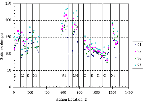
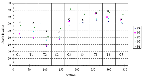
A plot of the static k-value determined for the Nevada site for years 1994 through 1997 from the basin test data is shown in figure 63. Note that the k-value reported is the composite value, which takes into account both the existing subgrade and the 7.6-cm granular subbase layer. Further, the values reported in the plot are static k-values obtained by multiplying the backcalculated value by 0.5.
Figure 63. Static k-values for Nevada test section.
1 psi = 6.89 kPa
1 m = 3.28 ft
It can be noted from figure 63 that the subgrade k-value continually changes from one end of the site to the other. For example, the mean k-values of the C2, L2, S2, and M2 sections are approximately at the same level and are lower than the mean k-values for the SA1 and LO1 sections. Further, there does not seem to be a clear time-series trend to the subgrade values between the various years of testing. The k-value ranges from 517 kPa to about 1,724 kPa (75 psi to about 250 psi) if the entire site is taken into consideration. This could potentially cause significant differences in the pavement responses along the test section.
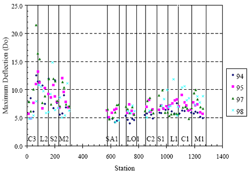
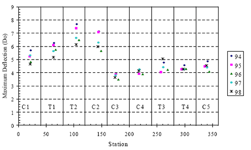
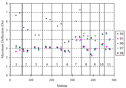
In figure 64, the variation of the maximum pavement deflection, Do, measured from the basin test, was plotted for the various treatment sections. Each year in which the data was collected was plotted as a separate series. It can be seen from the figure that Do varies greatly from section to section and from year to year. Comparing figures 63 and 64, the main cause of variation between the sections appears to be due to differences in subgrade support. For example, it can be noted from figure 63 the static k-value for the SA1 and LO1 treatment sections have the highest value for subgrade support. Thus, it is not surprising that these sections have the lowest deflection. However, what is unexpected is that the average deflection for each section appears to be decreasing slightly from year to year. Thus, the Do parameter does not appear to have any orrelation with the observed map cracking, which was noted to be increasing with time.
Figure 64. Nevada test site—Do from center slab.
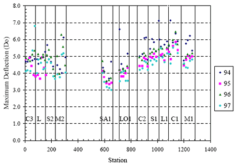
(Station location is in feet; 1 m = 3.28 ft)
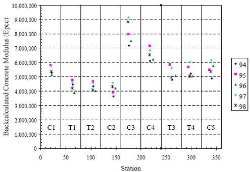
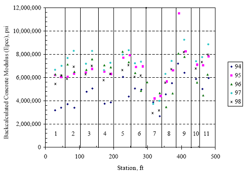
Figure 65 presents the section-to-section and year-to-year variation of backcalculated EPCC for the Nevada site. Unlike the center slab Do data, the backcalculated EPCC data shown in the figure is relatively consistent between the sections throughout the site. Because the k-value is accounted for in the backcalculation process, the difference in subgrade support conditions does not cause the large section-to-section variability seen with the Do parameter. Further, unlike what was found from laboratory modulus testing, no significant difference was noted in the modulus values between sections located on the east end (C1, C2, L1, M1, and S1) and west end (C3, L2, M2, S2) of the test site. However, the times series trends show that the average EPCC for each section increases slightly with time. This trend is contrary to what was expected, since the increase in map cracking over time should result in a lower EPCC.
Figure 65. Nevada test site—EPCC from center slab.
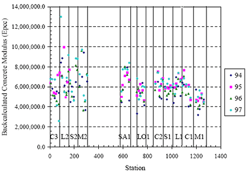
(Station location is in feet; 1 m = 3.28 ft)
Note that in figure 65, the values of EPCC range from 27,579 to 55,158 megapascals (mPa) (4 to 8 million psi). These numbers are higher than the previously reported laboratory values and also are relatively high for a pavement showing medium-to-high severity map cracking. However, it should be kept in mind that the backcalculated moduli do not necessarily agree with laboratory values since the loading rates and test conditions are quite different. Further, in backcalculating the pavement layer moduli, constant pavement and base layer thicknesses were assumed for the pavement layer—an assumption seldom realized in the field due to construction variability. However, despite these discrepancies, the higher EPCC values should not be of concern since only the relative change of modulus along the project and between the various testing instances is being evaluated.
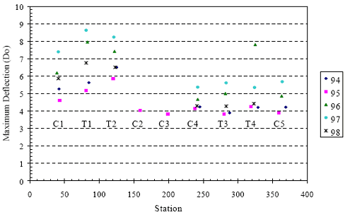
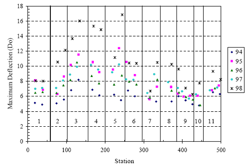
The Do data collected on the leave side of the joint, shown in figure 66, remained relatively consistent throughout the 5-year period. Some variation was identified between the years, but Do was increasing in some years and decreasing in others. The variation in Do appears to be temperature-related rather than ASR-related. No trend of increasing Do with time was observed, belying expectations. Thus, this parameter did not correlate with the observed joint distress data, which was increasing with time. However, as expected, the mean Do values for each treatment section were relatively greater than those at the mid-slab location.
Figure 66. Nevada test site—Do from leave side; deflection LTE (wheelpath).
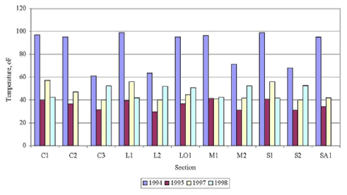
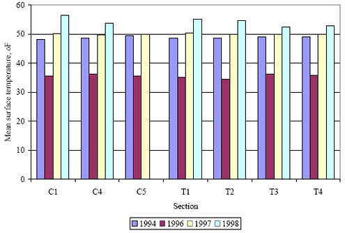
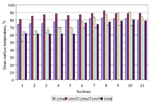
The average joint load transfer data for each treatment section is plotted in figure 67 for each year in which testing was conducted. The LTE values do not show a downward trend corresponding to the increased joint distress, as was noted in figure 10. LTE values range from approximately 30 to 88 percent with a significant amount of the data above 50 percent. The higher LTE values are inconsistent with a deteriorated, undoweled joint. A careful examination of the data revealed that the temperature at the time of testing was major confounding factor affecting the LTE values computed and can be used to explain some of the inconsistent and highly variable results. The average temperatures at the time of FWD testing for each treatment section are presented in figure 68. Ideally, the pavement temperature should be relatively constant for the entire data collection effort to make valid comparisons.
However, this condition seldom is realized in the field. It can be noted from figure 68 that the temperature varied from section-to-section during each visit (with some years, such as 1994, having a higher fluctuation than the others) as well as between visits. Comparing the temperature at the time of testing with the deflection LTE along the project length, it can be observed that the higher LTE values correspond to the higher test temperatures and vice versa. This is expected since the joints lock up at the higher test temperatures and produce higher load transfer values.Further, the fluctuation of the LTE values for each section seem to correlate more with the temperature at testing than any change in the real condition of the pavement.
Figure 67. Average LTE values for the various treatment sections for the Nevada site.
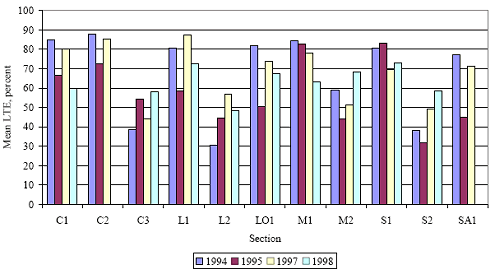
Figure 68. Average temperatures at time of joint testing for the Nevada site.
°C = (°F-32)/1.8
The test section in Newark, DE, was a relatively short section with a total project length of approximately 109.8 m. Only one type of treatment (lithium hydroxide—LIOH) was applied to this site to mitigate the ASR, and its performance was compared with side-by-side control sections. In all, there were four treatment sections (T1 through T4) and five control sections (C1 through C5). A description of the test section layout and the differential drainage conditions was presented in earlier sections of this report.
All of the Delaware data, with the exception of data from 1995, was collected using the standard sensor spacing described in the introduction. The 1995 data was also collected with the standard sensor spacing with the exception that the (12, 0) side sensor was not used. The Delaware testing locations consisted of one center slab and one leave side LTE test point per treatment in each year. An exception to this was that the C2 and C3 sections for LTE locations were not tested in 1995. Also, the LTE test points for the C5 section could not be collected in 1998. The various conclusions drawn from analyzing this data are presented below.
The variation of the subgrade support along the project was analyzed as a first step. Figure 69 presents a plot of the static subgrade k-value for the various sections.
Figure 69. Static k-values for the Delaware site.
(Station location is in feet; 1 m = 3.28 ft)
The static k-values were derived from the dynamic values obtained from backcalculation by multiplying the latter by a factor of 0.5. Note that the layout of the sections in the figure is the exact sequential order in which they are arranged in the field. It can be observed from the figure that the site can be divided into two groups based on the spatial variability of the k-values. The group with sections C1, T1, T2, and C2 has a lower mean k-value than the group with sections C3, C4, T3, T4, and C5. Also, there is some variability in the data on a year-to-year basis within each section. Overall, the k-values ranged from 414 to 1,103 kPa/2.54 cm (60 to 160 psi/inch).
The variation of the maximum pavement deflection, Do, measured from the center slab test is plotted in figure 70 for the various treatment sections. Section-by-section analysis of the data revealed that the C2, T1, T2, and C2 sections have a substantially higher Do than the other test sections. This result does correspond to the observed distress data, which also showed higher level of map cracking in these areas. This can be explained by the drainage and subgrade conditions. As described in the visual distress portion of this report, the first few sections of the Delaware test site were located in the low portion of a sag vertical curve and thus were exposed to more water during the wet months. This higher exposure could have weakened the pavement layers and increased the potential for materials-related distresses, including ASR. Further, as noted in figure 69, static mean k-value for this group of sections is lower than that for the remaining sections. This could be due to poor drainage or soil conditions. Regardless of the cause, the lower k-values could also have led to poorer structural performance.
Figure 70. Delaware test site—Do from center slab test.
(Station location is in feet; 1 m = 3.28 ft)
It can be noted from figure 70 that Do varies slightly from year to year. When each section was analyzed individually on a year-to-year basis, Do remained relatively constant for most sections, with some sections showing a slight downward trend. This result is contrary to the observed distress data, which shows map cracking is increasing with time. Variations in layer thicknesses, which were assumed to be constant in the backcalculation procedure, and variations in subgrade support conditions are likely responsible for this apparent discrepancy.
Figure 71 shows the variation of the EPCC along the section. Once again, there is a clear distinction in the modulus values of sections C1, T1, T2, and C2 compared to the remaining sections. The modulus values for these sections are lower and, as explained before for the Do data, are perhaps influenced by the map cracking prevalent in these sections. A similar trend was observed from the laboratory tested modulus values. However, the absolute magnitudes of the backcalculated moduli are far greater than their laboratory counterparts.
An examination of the time series data reveals that, similar to the Do pavement response, the backcalculated EPCC remained relatively constant with time. A few sections showed a slight upward trend with time. Based on these results, the EPCC parameter is not able to pick up on the observed data, which shows map cracking to be increasing with time. Thus, map cracking is not affecting the apparent structural capacity of the pavement, or more likely, the effects of slight variations in layer thickness and subgrade support conditions are interfering with the FWD’s ability to distinguish between the different levels of map cracking observed in this section.
Figure 71. Delaware test site—EPCC from center slab.
(Station location is in feet; 1 m = 3.28 ft)
Figure 72 presents the variation of the maximum deflection data collected at the joints along the Delaware site. The data in the figure suggests that Do did show a slight increasing trend with time from 1994 through 1997. However, the measured Do dropped sharply in 1998, and overall the leave side Do response did not reveal a difference between the treated and the non-treated sections. For the Delaware test site, both the FWD data and the observed distress data indicated that the drainage differences between the sections has a far greater influence on pavement performance than the treatment type.
Of the four pavement response parameters analyzed, Do on the leave side of the joint showed the best correlation with the observed joint distress data. A statistical analysis consisting of a Duncan grouping was performed on this data. Because the Delaware site contained only one test point per section, the data from all years was grouped together. The Duncan grouping confirmed that the Do parameter mirrored the observed joint distress data. The observed data showed that sections in the poor drainage areas of the site exhibited the highest levels of joint distress. Likewise, the Duncan grouping showed that maximum mean deflection for treatment sections C1, T1, and T2 were higher than and statistically different from the maximum mean deflections in sections C4, C5, T3, and T4. The results of the Duncan grouping are shown in table 48.
Figure 72. Delaware test site—Do from leave side.
(Station location is in feet; 1 m = 3.28 ft)
| Treatment | Mean Leave Side Do | Duncan Grouping |
|---|---|---|
| T1 | 7.24 | A |
| T2 | 7.16 | A |
| C1 | 6.18 | A,B |
| T4 | 5.44 | C,B |
| C5 | 4.92 | C,B |
| T3 | 4.70 | C |
| C4 | 4.64 | C |
The variation of the LTE values along the project is presented in figure 73. The LTE data is presented both on a yearly and treatment section basis. In both cases, the calculated LTE values remained relatively constant. The magnitudes of the LTE values were also in the high range (between 70 and 90). This is not a totally unexpected finding since most of the joint deterioration (spalling) observed was of low severity. It is possible that the low severity spalling did not cause deterioration to an extent that would destroy the LTE at the joints. Further, unlike the Nevada section, temperature was not a confounding variable. Figure 74 presents the average testing temperature for each year in which the survey was performed. It can be observed from the figure that the temperature was fairly consistent between visits, as well as from the first to the last section during each visit.
Figure 73. Delaware test site—LTE.
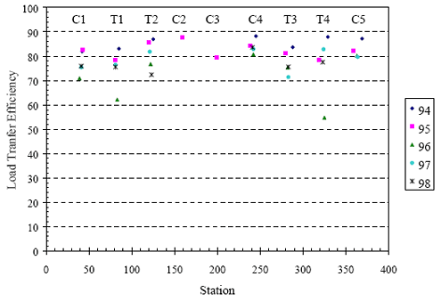
(Station location is in feet; 1 m = 3.28 ft)
Figure 74. Average temperatures at time of joint testing for the Delaware site.
°C = (°F-32)/1.8
The test temperatures in all the years were below 15.56 °C, reducing the possibility of the joint lockup.
As noted earlier in the report, the California site had two experimental sites. One of the sites was an overhead structure, and the other was a conventional highway pavement. The pavement test sections were constructed in the early 1970s and had undergone an ASR mitigating treatment in the form of a methacrylate coating. The site consists of three sections coated with methacrylate (M1, M2, and M3) and three control sections (C1, C2, and C3). Figure 38 presented details of the section layout. FWD testing was performed on sections C1, M1, and M2, which are located in the passing lane. The treatment section M2 received an additional coating of the methacrylate in 1995. As noted in table 47, the sections consist of a 21.0-cm PCC layer resting on a 10.2-cm cement-treated base.
The testing locations contained a minimum of nine test points in the control section and at least eight test points in each of the methacrylate treated sections. Some years contained additional test points in various locations. For data analysis purposes, the data collected on 2/28/95 was designated as 1994 data. Center slab data was analyzed for each of the years 1994 through 1998. Joint test data was analyzed for 1994, 1997, and 1998. The 1995 joint data was not included in the analysis because only the approach side of the joint was tested in 1995. However, this omission is not expected to pose any significant problems in evaluating the performance of the test sections. The 1996 joint data could not be collected due to weather-related problems, as noted earlier.
The variation of the subgrade support along the project was analyzed as a first step. Figure 75 presents a plot of the static subgrade k-value for the various sections. It can be observed from the figure that the control section C1 has a higher k-values on an average compared to the methacrylate sections M1 and M2. The mean k-value of section C1 is approximately 1034 kPa/2.54 cm (150 psi/inch) with a range of 689 to 1,379 kPa (100 to 200 psi), whereas the mean k-value for treatment sections M1 and M2 is approximately 517 kPa (75 psi) with a range of 345 to 689 kPa/25.4 cm (50 to 100 psi/inch). Further, the variability in the k-value on a yearto- year basis is higher for the treatment section C1 than for M1 and M2. These observations will likely assume significance in evaluating the FWD data.
Figure 76 shows a plot of the variation of the maximum mid-slab deflection, Do, along the project length. As expected, the control section, which had a lower subgrade support value, also had higher average deflections than treatment sections M1 and M2. Also, the Do varies greatly from year to year. Because of this variation, no clear trend of increasing or decreasing deflection in relation to time could be identified.
Figure 75. Static k-value for California test section.
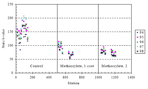
(Station location is in feet; 1 m = 3.28 ft)
Figure 76. California test site—Do from center slab.
(Station location is in feet; 1 m = 3.28 ft)
Rather, Do remains relatively constant over the 5-year testing period, and because of this, no correlation between center slab deflection and map cracking could be developed.
The backcalculated concrete modulus is plotted against station location in figure 77. Similar conclusions can be drawn from this figure as from the Do data. The mean EPCC values are relatively consistent between the treatment sections and over time. There appear to be some spurious deflections in the dataset that result in unrealistic numbers for the EPCC. But if these points are discounted, the EPCC for all the sections range from 27,579 to 55,158 mPa (4 to 8 million psi), which is still relatively high for an old pavement section showing signs of ASR. It was noted from coring data that the thickness of the pavement sections varied along the project length, with some sections substantially thicker than the 21 cm adopted in backcalculation. This could be a plausible explanation for the higher EPCC values.
Figure 77. California test site—EPCC from center slab.
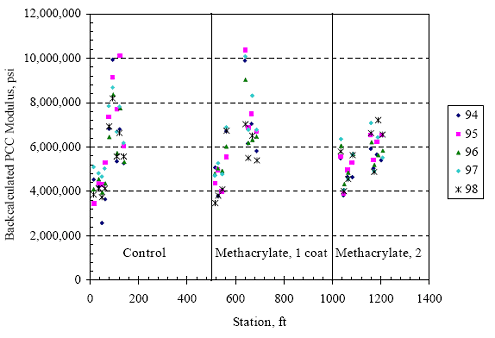
1 psi = 6.89 kPa
1 m = 3.28 ft
This discrepancy in the magnitudes of modulus values, nevertheless, does not diminish the value of the data presented since only relative trends were being examined here in an effort to correlate EPCC with the amount of map cracking. Based on the data presented there does not appear to be a consistent time-series trend to the modulus values. It was expected that the modulus values will drop with time corresponding to the proportional increase in map cracking. It may be that, just as with Do at the mid-slab location, the backcalculated moduli are not sensitive to the map cracking since most of the distress at mid-slab was at low severity.
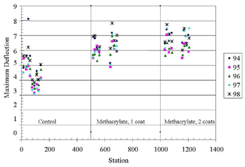
An analysis of the maximum joint deflection data shown in figure 78 showed that the Do values have a slight increasing trend over time. However, the differences were relatively slight and are not proportional to the increase in the amount of observed joint distress data. Overall, the levels of maximum joint deflection were about double the maximum interior deflection (mid-slab values), which is as expected. An examination of the average values for each section revealed that the methacrylate 1 section had the highest deflection, followed by the control and the methacrylate 2 sections. It is difficult to postulate what the expected joint deflection over time is expected on jointed pavement having ASR distress. In jointed pavements, without dowels, joint deflection and curling can be large. As ASR develops, the concrete expands reducing joint openings and increasing aggregate interlock across the joint. Joint curling is essentially eliminated and the ride (smoothness) is improved.
As ASR deterioration continues, spalling and loss of integrity at the joints occurs. However, even though the concrete is disintegrating, the joints remain very tight.
Figure 78. California test site—Do from leave side.
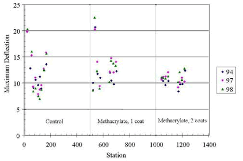
(Station location is in feet; 1 m = 3.28 ft)
The variation of the LTE along the project is shown in figure 79. Although the load transfer efficiencies are relatively high, the LTE has the best correlation with the observed joint distress data. The average values for each section decrease substantially from 1994 through 1997. There is a slight increase in the LTE from 1997 to 1998 in the methacrylate 1 and control sections, but this is expected given the temperature at the time of testing. For these sections, the test temperature in 1998 was approximately 10 degrees higher than in 1997. For the methacrylate 2 section, the 1997 and 1998 test temperatures were approximately equal, and the LTE continued to decrease. Ranking the average LTE for each section shows the expected correlation with the joint distress data. The methacrylate 2 section has the highest average LTE, followed by the methacrylate 1 section, followed by the control section. A statistical analysis was performed to determine if the difference in LTE between the treatment types was significantly different. This analysis consisted of a Duncan grouping at an alpha level of 0.05. This analysis confirmed that the LTE for the methacrylate-treated sections was significantly higher than the LTE for the control section. The results of the Duncan grouping are shown in table 49.
Figure 79. California test site—LTE.
(Station location is in feet; 1 m = 3.28 ft)
| 1994 | ||
|---|---|---|
| Treatment | Mean LTE | Duncan Grouping |
| Methacrylate, 2 | 84.3 | A |
| Methacrylate, 1 | 80.0 | A |
| Control | 63.9 | B |
| 1997 | ||
| Treatment | Mean LTE | Duncan Grouping |
| Methacrylate, 2 | 73.0 | A |
| Methacrylate, 1 | 69.5 | A |
| Control | 52.0 | B |
| 1998 | ||
| Treatment | Mean LTE | Duncan Grouping |
| Methacrylate, 2 | 73.3 | A |
| Methacrylate, 1 | 71.3 | A |
| Control | 61.5 | B |
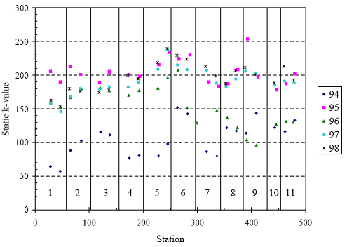
The New Mexico test pavement was built specifically to support SHRP ASR research. Details regarding the section layout and treatment types were explained in earlier sections. The pavement is 20.3 cm thick with a 15.2-cm cement-treated base layer. Two different aggregate sources were used in the construction of the various test sections. Class C and F fly ash and lithium hydroxide were the main ASR mitigating treatments. Side-by-side control sections were also provided for comparison. In all, 11 treatment sections were available for comparison. The sections are numbered from 1 through 11 as shown in figure 55.
The New Mexico test locations for the center slab testing consisted of two test points per treatment, except for section 10, which contained only one test point. The test locations for the LTE testing consisted of two test points per treatment with the exception of sections 8, 9, and 10. Sections 8 and 10 contained one test point in each year, and section 9 contained three test points in each year. All data was collected using the standard sensor spacing described earlier.
A plot of the variation of the backcalculated subgrade support value along the project is presented in figure 80 for each year the data was collected. The subgrade support value is relatively constant within each visit and between visits for the years 1995, 1997, and 1998. The mean k-value for the various sections based on this data is 1,379 kPa/2.54 cm (200 psi/inch). The k-value is quite variable in 1994 and 1996, with the lowest k-values being recorded in the former year. The type of subgrade soils present at the site location and the saturation state of the soils during the time at which the FWD testing was conducted could likely explain these findings. For example, an intense rainfall event a few days prior to the testing in combination with a moisturesensitive subgrade soil and poor drainage conditions could lead to a weak subgrade support condition. However, actual occurrence of this event could not be ascertained from the data collected.
In figure 81, the project variation of Do is presented for the multiple years in which data was collected. From this figure it can be seen that Do varies greatly, especially for the 1994 data. The Do values follow the expected trends based on the subgrade support conditions shown in figure 80. It seems likely that saturated subgrade conditions were present during the 1994 data collection. This would explain the substantially higher Do values obtained for that year.
An examination of the data on a section-by-section basis and on a year-to-year basis did not indicate any clear trend regarding Do. There does not appear to be any apparent correlation between Do and map cracking for this section. Recall that map cracking has been reported to increase in all sections between 1994 and 1998, with the exception of sections 3 and 4; with the last 2 years registering a dramatic increase. However, most of the map cracking reported was of low severity, and it is assumed that the FWD test was not sensitive enough to register this distress.
Figure 80. Static k-value for New Mexico test.
(Station location is in feet; 1 m = 3.28 ft)
Figure 81. New Mexico test site—Do from center slab.
(Station location is in feet; 1 m = 3.28 ft)
In figure 82, the backcalculated EPCC is plotted for all the treatment sections. Similar to the Do pavement response, the backcalculated EPCC remained relatively constant over time. Based on these results, the EPCC parameter is not able to corroborate the observed distress data, which shows map cracking to be increasing over time. Thus, the map cracking is not affecting the apparent structural capacity of the pavement, or more likely, the effects of slight variations in layer thickness and subgrade support conditions are interfering with the FWD’s ability to distinguish between the different levels of map cracking observed in this section.
Figure 82. New Mexico test site—EPCC from center slab.
1 psi = 6.89 kPa
1 m = 3.28 ft
Figure 83 presents the maximum pavement deflection collected from joint testing. As with the Do center slab data, the Do data taken from the leave side of the joint showed rather large variability. Overall, the data did show a slight upward trend over time corresponding to increased joint distress. However, this trend was not consistent, as the data was confounded by differences in temperatures at testing between sections during each visit. A pictorial representation of the average temperature at the time of FWD testing for each section is presented in figure 84. Other confounding factors include variations in slab thickness due to construction variability and changing subgrade support conditions.
Figure 83. New Mexico test site—Do from leave side.
(Station location is in feet; 1 m = 3.28 ft)
Because the Do data did at least show the expected trend of increasing with time, a statistical analysis was performed. This analysis revealed some differences between the treatment types; however, these differences appear to be more closely related to temperature and subgrade support conditions than to ASR-related deterioration.
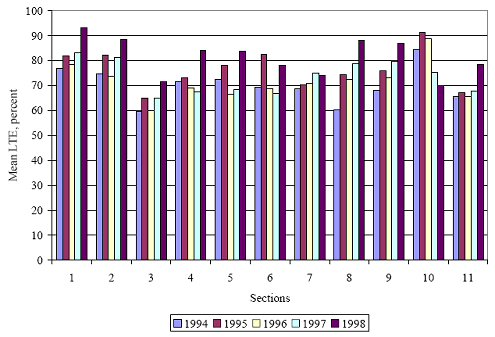
The variation of the LTE along the project is plotted in figure 85. An examination of the LTE data on both a yearly and section-by-section basis revealed that LTE remained relatively constant. The LTE data did not have a significant correlation with the observed joint distress data, and it could not be used to corroborate the benefit of the Class F fly ash treatment. A statistical analysis revealed that the average LTE values for each section belonged to the same group. Thus, no significant differences in LTE values existed between any of the treatment types.
Figure 84. Temperature variation during FWD testing for the New Mexico site.
°C = (°F-32)/1.8
Figure 85. New Mexico test site—LTE.
Visual surveys confirmed that each of the four experiment sites were accumulating increased amounts of ASR-related distress over the 5-year experiment time frame. It was hoped that correlations could be developed which would relate pavement responses collected by the FWD to the observed ASR–related distresses. To assess the FWD’s ability to identify ASR relateddistress, four pavement response parameters were examined in detail: maximum deflection and backcalculated modulus collected from center slab tests, and Do and LTE collected from joint tests. It was believed that these four parameters offered the best chance to develop a meaningful correlation to the observed distress data. Attempts were made to correlate center slab Do and EPCC to the map cracking data. It was expected that Do would increase and that EPCC would decrease as the observed map cracking increased.
Attempts were also made to correlate Do and LTE measured at the joints to the observed joint distress data. It was expected that Do would increase and that LTE would decrease in relation to observed increase joint distress severity.
Based on the analysis results, no significant correlations could be developed linking the FWD data to the observed distresses, particularly when the distresses were of low severity. For all four sites, center slab Do and EPCC proved to be very poor indicators of ASR–related map cracking. In each of the four sites, Do and EPCC remained relatively constant over time, and differences between treatment sections at any given site were found to correlate with variations in subgrade support conditions, rather than to the observed differences in map cracking. Further complicating the EPCC analysis is the issue of slight variations in layer thickness. It seems apparent that the effects of subgrade support, temperature, and possible variation from assumed layer thickness far outweigh the FWD’s ability to distinguish between varying levels of map cracking.
FWD data collected from joint tests was slightly more promising. The LTE data from the California site correlated well with the observed joint distress data, as did the Do data from the Delaware site. However, these results are far from conclusive, and overall, the majority of the joint data did not correlate well with the observed distress.

