U.S. Department of Transportation
Federal Highway Administration
1200 New Jersey Avenue, SE
Washington, DC 20590
202-366-4000
Federal Highway Administration Research and Technology
Coordinating, Developing, and Delivering Highway Transportation Innovations
 |
| This report is an archived publication and may contain dated technical, contact, and link information |
|
Publication Number: FHWA-HRT-10-065 Date: December 2010 |
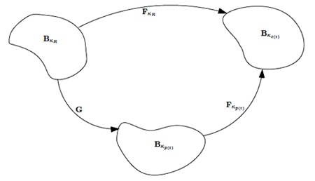
The framework this study adopts to model asphalt concrete recognizes that, corresponding to any current configuration of a body, several associated natural configurations are possible. Of these natural configurations, the body may go to one specific natural configuration when the tractions are removed, preferably a stress-free state (see figure 3).
Figure 3. Illustration. Evolution of natural configurations associated with microstructural transformations resulting from the material response to an external stimulus.
The specific natural configuration that the body goes to depends on the process. For example, perfectly elastic materials have a unique stress-free configuration, deferring only by a rigid body motion from each other. During deformation, the underlying microstructural mechanism does not change, and the body returns to the same stress-free state on the removal of applied traction. For a classical viscoelastic material capable of instantaneous elastic response, the stress-free state obtained by an instantaneous elastic unloading response can be associated with a natural configuration. To develop a model for HMA capable of representing the transformation of the mix (i.e., a low-viscosity fluidlike state to a high-viscosity fluidlike state), researchers began with the same assumption by associating the natural configuration of the material with the stress-free state obtained upon instantaneous elastic unloading. The model developed is an isothermal, compressible, viscoelastic, nonlinear fluidlike model. The chief constitutive assumptions for the model are presented briefly, and further details regarding model development have been published elsewhere.(48,49)
The material model developed has to satisfy the second law of thermodynamics in the form of the energy-dissipation inequality shown in figure 4.
Figure 4. Equation. Energy-dissipation inequality.
Splitting the entropy production into two parts—that due to thermal effects and that due to mechanical dissipation—and requiring both of them to be individually nonnegative leads to the equation in figure 5.
Figure 5. Equation. Reduced energy-dissipation inequality.
In the current model, temperature is assumed to be constant during laboratory compaction. In general, the temperature effect can be accounted for by allowing the material parameters in the constitutive model to be different at different temperatures.
The specific Helmholtz potential for a solid, ψ, is given in figure 6.
Figure 6. Equation. Helmholtz potential for mixture.
The rate of dissipation due to the mechanical working ![]() is specified in figure 7.
is specified in figure 7.
Figure 7. Equation. Rate of dissipation function.
Since the mixture is considered a single constituent, the shear-modulus function, μ, can be thought of as a material property that reflects the characteristics of the aggregate matrix, and the viscosity function, η, reflects the characteristics of the asphalt mastic. Such a specification of the rate of dissipation corresponds to a material with a power-law-type viscosity and is therefore used to model the non-Newtonian fluidlike nature of the mix. During compaction, the aggregate matrix, which is initially in a loose form, slowly evolves into a dense aggregate matrix. This densification is further aided by the changes in the asphalt mastic due to densification and reduction of mastic film thickness. The specific forms for the shear-modulus and viscosity functions chosen (figure 8 and figure 9) represent such evolution.
Figure 8. Equation. Shear-modulus function.
Figure 9. Equation. Viscosity function.
To take into consideration the highly compressible behavior during the initial stages of compaction and the material hardening as it reaches the limits of compressibility toward the end of the compaction process, choices are made for μ and η in figure 8 and figure 9
Considering the form chosen for the Helmholtz potential and the rate-of-dissipation function, the constitutive form for stress is obtained in figure 10.
Figure 10. Equation. Constitutive equation for stress.
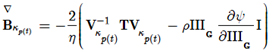
Figure 11. Equation. Evolution equation.
For validation of the model, consideration needs to be given to three-dimensional compressive deformation with applied static and dynamic loads. However, to do this, the model needs to be implemented in an FE methodology that will enable modeling the three-dimensional behavior in general. Therefore, researchers chose to study the developed model through analytical calculations aided in part by the computations. Presented in this section are the formulation for such a study and the calculations performed using numerical computation software MATLAB®.(52)
The governing equations of motion for the constrained one-dimensional compression of the material model were developed using a semi-inverse approach by prescribing the necessary deformation field for this case. The model's response to constant stress and constant strain is illustrated in the following sections.
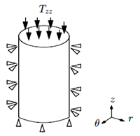
The diagonal components of stress are unknown except for the prescribed creep load (see figure 12). Hence, a constant compressive stress is applied along the axial z-direction.
Considering that the specific application is a one-dimensional constraint creep, the axial stress and other similar dimensional quantities can be normalized using the initial applied creep load.
Figure 12. Illustration. Schematic for the one-dimensional compression problem.
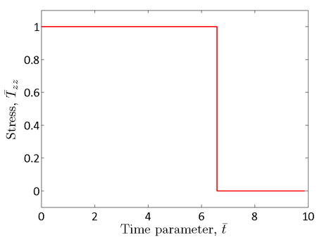
Typical plots obtained for the given material by calculating the solution to the semi-inverse creep problem using MATLAB® are depicted in figure 13 through figure 18. Kinematical terms are nondimensional quantities. The material model is subject to a sudden normal stress, and the deformation response shows the viscoelastic nature of the material.
Figure 13. Chart. Creep solution for the material model for HMA—creep load.
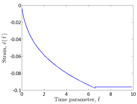
Figure 14. Chart. Creep solution for the material model for HMA—Almansi strain.
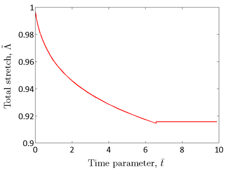
Figure 15. Chart. Total stretch calculated from the solution to the one-dimensional creep problem.
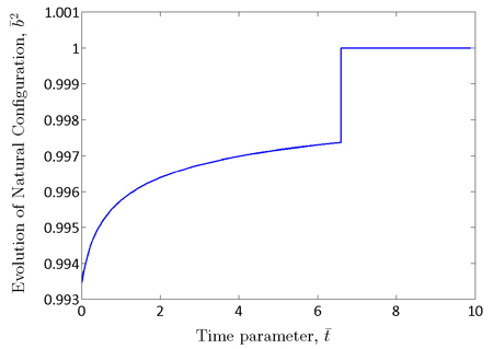
Figure 16. Chart. Evolution of natural configuration calculated from the solution to the one-dimensional creep problem.
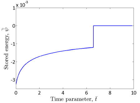
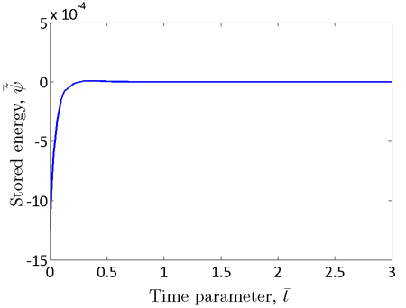
Figure 17. Chart. Stored energy calculated from the solution to the one-dimensional creep problem.
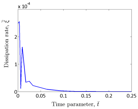
Figure 18. Chart. Rate of dissipation calculated from the solution to the one-dimensional creep problem.
Strain lags behind stress because of the material's viscoelasticity. Upon instantaneous removal of the load, the material rebounds partially to attain a permanent strain. Plots of some of the relevant field variables calculated after obtaining the solution are presented in figure 15 through figure 18. All quantities have been nondimensionalized. The nondimensionalized stored energy has negative values due to the nondimensionalization of shear modulus with respect to the initial applied load. The stored energy starts high and then, as the material evolves, dissipates (though the rate of dissipation decreases) to none upon unloading. The natural configuration of the material evolves as well during the process, and its evolution is presented in figure 16. The plot shows that the material returns to a natural (stress-free) configuration upon unloading; therefore, the dissipation occurs because of a change in the microstructure of the material.
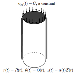
Similarly, researchers solved for the motion of the one-dimensional deformation under a constant applied strain (i.e., with respect to the current configuration) and observed the corresponding stress response as a function of time (see figure 19).
Figure 19. Illustration. Schematic for the one-dimensional stress-relaxation problem.
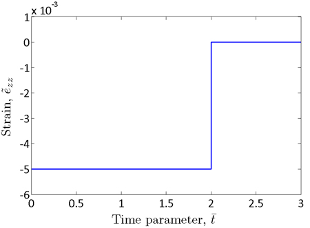
The calculations of the response of the model to a step-input strain results in the characteristics shown in figure 20 through figure 23. All quantities have been nondimensionalized.
Figure 20. Chart. Applied strain calculated from the solution to the one-dimensional stress-relaxation problem.
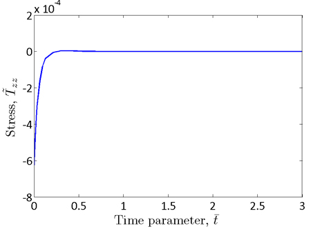
Figure 21. Chart. Stress relaxation calculated from the solution to the one-dimensional stress-relaxation problem.
Figure 22. Chart. Stored energy calculated from the solution to the one-dimensional stress-relaxation problem.
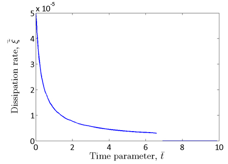
Figure 23. Chart. Rate of dissipation calculated from the solution to the one-dimensional stress-relaxation problem.
The applied compressive strain is 0.005, and the resultant nondimensionalized stress response depicted in figure 20 through figure 23 shows that the stress relaxes slowly and reaches a stress free state. The stress-free state is reached after the material dissipates the energy it stores to change its microstructure. Again, the nondimensionalized stored energy has negative values due to nondimensionalization.
Therefore, the material model predicts the expected response to mechanical loads for compressible, viscoelastic material models.