U.S. Department of Transportation
Federal Highway Administration
1200 New Jersey Avenue, SE
Washington, DC 20590
202-366-4000
Federal Highway Administration Research and Technology
Coordinating, Developing, and Delivering Highway Transportation Innovations
 |
| This report is an archived publication and may contain dated technical, contact, and link information |
|
Publication Number: FHWA-HRT-10-065 Date: December 2010 |
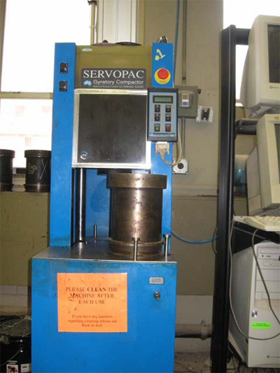
In the laboratory, the compaction process takes place at high temperatures (see figure 37 for an example of the equipment used). Some phenomena and parameters necessary for the model only occur or are only relevant at higher temperatures. This makes it impossible to conduct conventional laboratory testing of specimens (e.g., triaxial testing) to obtain these parameters. This limitation was overcome by implementing the mathematical model in finite elements, conducting simulations of the SGC compaction process, and then fitting the FE results to the available data in the form of SGC curves to determine the model parameters. These parameters were then considered to include the information necessary to characterize material behavior under various conditions. Assuming that the material in the laboratory is representative of that in the field, the model parameters obtained from the SGC calibration can be used to simulate field compaction under loading and boundary conditions in the field (see figure 38 for an example of field rolling compaction). This does not imply that the SGC process can be assumed to be the same as field compaction.
Figure 37. Photo. Superpave® gyratory compactor.
Figure 38. Photo. Static steel-wheel roller.
Once the model input parameters were identified, correlations to material properties could be found. It was expected that the model input parameters would be influenced by the following material properties:
Model Verification and Calibration
Several studies have been conducted into the experimental characterization of the influence of different laboratory and field compaction procedures on the internal structure of asphalt mixtures and their mechanical properties. From these studies, the following information and materials can be used in verification and calibration:
Available data were used to determine the relationship between mixture properties, temperature, and model parameters. The model parameters were determined by calibrating the FE model to match the SGC curves. This was followed by verification of the FE implementation's prediction using a set of data that was not used in the model calibration. Field compaction measurements were used for further calibration and validation. FE models that simulate the loading and boundary conditions in the field were developed. The model parameters that were determined using the laboratory calibration were used initially in the field FE models. Calibration was introduced as needed to better simulate the field compaction. Such calibration was necessary to account for possible differences in materials between the laboratory and the field.
The FE implementation of the model developed was used to simulate the compaction processes and the simulated compactor response, and changes in mixture stiffness at different stages of compaction were compared to the measured response and mixture stiffness.
The constitutive model developed was incorporated into two FE programs, Abaqus (a commercial FE package) and CAPA-3D. The constitutive model was implemented in Abaqus through the user material subroutine, UMAT.(2) The CAPA-3D general structure has been presented in detail by Scarpas.(53,54) For the implementation of the present model, CAPA 3D required the input of two interface subroutines that provide the system with the necessary model parameters and the algorithm for the required stress updates at each material point. The required equations were obtained through a numerical discretization of the material constitutive relations of the model to obtain a system of nonlinear algebraic equations at each material-integration point. The computational sequences were then provided in the interface subroutines in the form of Fortran code. Further details on the usage of the computational system are provided in the CAPA-3D user manuals.(53,54)
The SGC was simulated through a lateral constraint along the boundary and a constant vertical stress of 87 psi (600 kPa). In addition, sinusoidal vertical displacements that were 120 degrees out of phase were applied at equidistant locations around the periphery of a plate supporting the mix from the bottom. This was done to simulate the applied angle of gyration in the SGC, which is responsible for inducing shear in the mix. The frequency of the applied gyrations was 30 gyrations per minute. The bottom support plate was modeled as a nearly rigid material. Also, a constant friction factor of 0.4 was introduced between the mixtures and the plates and mold.
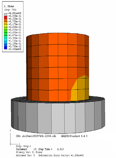
The compaction curves obtained from the simulations were plotted as the normalized height of the specimen versus time of compaction. The normalized height is defined as the height of the specimen at any time divided by the initial height of the mixture in the SGC. Figure 39 shows an example of the FE mesh of the SGC.
Figure 39. Illustration. FE mesh used in modeling the SGC.
A comprehensive parametric analysis was conducted in order to determine the sensitivity of the mixture compaction to the various models' parameters. The parameters that were used in this analysis are shown in table 2. All the SGC simulations were conducted using an angle of 1.25 degrees.
Table 2. Model parameters used in the parametric study.
Set No. |
|
λ1 |
n1 |
q1 |
|
λ2 |
n2 |
q2 |
|---|---|---|---|---|---|---|---|---|
1 |
1,700 |
0.22 |
4 |
−24 |
1,400 |
0.25 |
3 |
−30 |
2 |
1,900 |
0.22 |
4 |
−24 |
1,400 |
0.25 |
3 |
−30 |
3 |
1,500 |
0.22 |
4 |
−24 |
1,400 |
0.25 |
3 |
−30 |
4 |
1,700 |
0.25 |
4 |
−24 |
1,400 |
0.25 |
3 |
−30 |
5 |
1,700 |
0.20 |
4 |
−24 |
1,400 |
0.25 |
3 |
−30 |
6 |
1,700 |
0.22 |
5 |
−24 |
1,400 |
0.25 |
3 |
−30 |
7 |
1,700 |
0.22 |
3 |
−24 |
1,400 |
0.25 |
3 |
−30 |
8 |
1,700 |
0.22 |
4 |
−26 |
1,400 |
0.25 |
3 |
−30 |
9 |
1,700 |
0.22 |
4 |
−21 |
1,400 |
0.25 |
3 |
−30 |
10 |
1,700 |
0.22 |
4 |
−24 |
1,600 |
0.25 |
3 |
−30 |
11 |
1,700 |
0.22 |
4 |
−24 |
1,300 |
0.25 |
3 |
−30 |
12 |
1,700 |
0.22 |
4 |
−24 |
1,400 |
0.26 |
3 |
−30 |
13 |
1,700 |
0.22 |
4 |
−24 |
1,400 |
0.22 |
3 |
−30 |
14 |
1,700 |
0.22 |
4 |
−24 |
1,400 |
0.25 |
4 |
−30 |
15 |
1,700 |
0.22 |
4 |
−24 |
1,400 |
0.25 |
2.5 |
−30 |
16 |
1,700 |
0.22 |
4 |
−24 |
1,400 |
0.25 |
3 |
−26 |
17 |
1,700 |
0.22 |
4 |
−24 |
1,400 |
0.25 |
3 |
−34 |
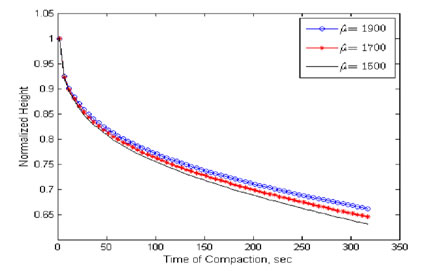
An example of the influence of ![]() , keeping all other parameters the same, is shown in figure 40. As expected, more compaction was achieved as
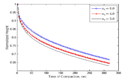
, keeping all other parameters the same, is shown in figure 40. As expected, more compaction was achieved as ![]() decreased. The effect of this parameter on the compaction process becomes more important at longer compaction times, when the mixture becomes more or less a highly viscous fluid. The analysis of parameter n1 (shown in figure 41) showed that μ is significantly affected by the n1 value (see figure 8), which controls the maximum compaction (change in height) of a mixture.
decreased. The effect of this parameter on the compaction process becomes more important at longer compaction times, when the mixture becomes more or less a highly viscous fluid. The analysis of parameter n1 (shown in figure 41) showed that μ is significantly affected by the n1 value (see figure 8), which controls the maximum compaction (change in height) of a mixture.
Figure 40. Chart. Analysis of the sensitivity of compaction to ![]() .
.
Figure 41. Chart. Analysis of the sensitivity of compaction to n1.
Analysis of the λ1 parameter revealed that mixture compaction is affected very little, if any, by this parameter within the range of 0.2 to 0.3. This specific range for λ1 is significant to obtain the initial viscous dissipation during the deformation. Therefore, λ1 was treated as a constant chosen to lie within this range in the model in order to simplify obtaining the remaining parameters. Another parameter that has a very small effect on the compaction process is q1. Therefore, this parameter was also treated as a constant in the model.
Figure 42 shows that the parameter ![]() controls the point at which the material behavior starts to change from a very low-viscosity fluidlike behavior (rapid compaction) to a highly viscous fluid behavior (slow compaction). In figure 42, the material with
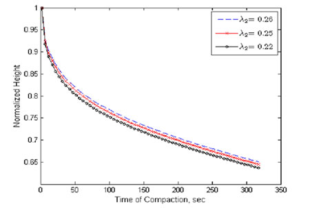
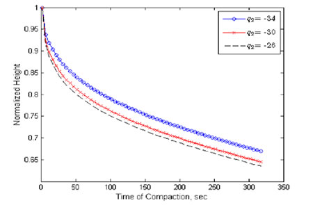
controls the point at which the material behavior starts to change from a very low-viscosity fluidlike behavior (rapid compaction) to a highly viscous fluid behavior (slow compaction). In figure 42, the material with ![]() = 232.06 ksi·s (1,600 MPa·s) experiences change in the compaction rate prior to the other two materials. The parameter λ2, presented in figure 43, is directly related to the initial slope of the compaction curve (initial viscosity of the mixture). As shown in figure 44, the model parameter q2 contributes to the nonlinear change of viscosity from the start of the compaction process, when the mixture exhibits low-viscosity fluidlike behavior. The overall compaction of the mixture is higher at lower (more negative) values of q2. The parametric analysis showed that n1 has almost no effect on the compaction curve when it lies between 2 and 4. Consequently, n1 is assumed to be a constant within this range for the SGC simulations presented in this chapter.
= 232.06 ksi·s (1,600 MPa·s) experiences change in the compaction rate prior to the other two materials. The parameter λ2, presented in figure 43, is directly related to the initial slope of the compaction curve (initial viscosity of the mixture). As shown in figure 44, the model parameter q2 contributes to the nonlinear change of viscosity from the start of the compaction process, when the mixture exhibits low-viscosity fluidlike behavior. The overall compaction of the mixture is higher at lower (more negative) values of q2. The parametric analysis showed that n1 has almost no effect on the compaction curve when it lies between 2 and 4. Consequently, n1 is assumed to be a constant within this range for the SGC simulations presented in this chapter.
Figure 42. Chart. Analysis of the sensitivity of compaction to ![]() .
.
Figure 43. Chart. Analysis of the sensitivity of compaction to λ2.
Figure 44. Chart. Analysis of the sensitivity of compaction to q2.
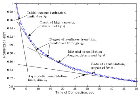
The equations for shear-modulus-like function μ and viscosity-like function η are represented in figure 45 and figure 46, respectively, after assigning constant values to λ1, q1, and n2.
Figure 45. Equation. Modified shear-modulus function.
Figure 46. Equation. Modified viscosity function.
The viscosity function primarily controls the initial compaction when the material behaves like a fluid with very low viscosity. The change in viscosity during compaction is associated with changes in the reduction in asphalt film thickness, leading to an increase in the overall viscosity of the mixture. On the other hand, the shear-modulus function primarily controls the compaction process after some compaction when the material starts to behave like a highly viscous fluid. The increase in the shear modulus is associated with changes in the aggregate structure due to the development of more contacts and interlocking.
Based on the parametric analysis and the physical significance of the model's parameters, the parameters are summarized as follows:
The relationship between the model's parameters and the compaction process is illustrated in figure 47.
Figure 47. Chart. Illustration of the relationship of the model's parameters to the compaction process.
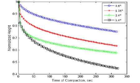
Figure 48 presents the results of FE simulations of the SGC at different angles of gyration. The model captures the influence of the angle on the change in compaction. Also, the compaction behavior does not change in a linear manner with the change in angle.
Figure 48. Chart. Influence of angle of gyration on the compaction curve.
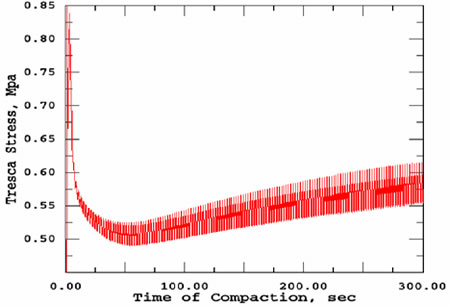
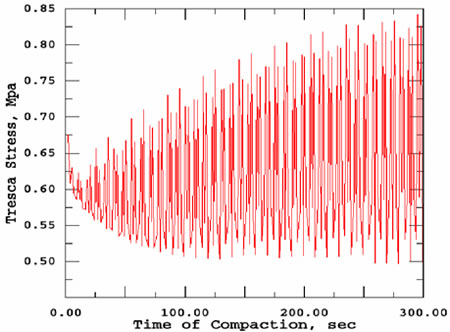
The FE model was used to determine the maximum shear stresses at the top of the specimens for angles of gyration of 1.25 and 2.0 degrees (shown in figure 49 and figure 50, respectively). The analysis was conducted using the model's parameters determined for the SH-36 mixture presented later in this report. Initially, the shear stress decreases rapidly when the material behaves as a compressible fluid and then starts to increase gradually as the mixture starts to behave like a highly viscous fluid. The shear stresses are higher for higher angles of compaction because an increase in the angle of gyration is associated with an increase in the applied shear stresses. Also, the point at which shear stress starts to increase occurs earlier at a 2.0-degree angle than at a 1.25 degree angle. This is because the mixture compacts and gains strength faster at a 2.0 degree angle of gyration.
Figure 49. Chart. Maximum shear stress at the top of the specimen for a gyration angle of 1.25 degrees.
Figure 50. Chart. Maximum shear stress at the top of the specimen for a gyration angle of 2.0 degrees.
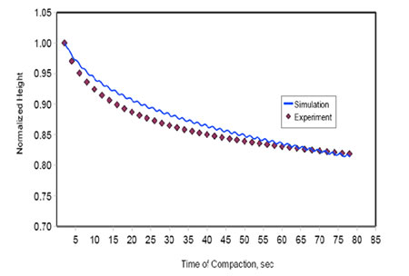
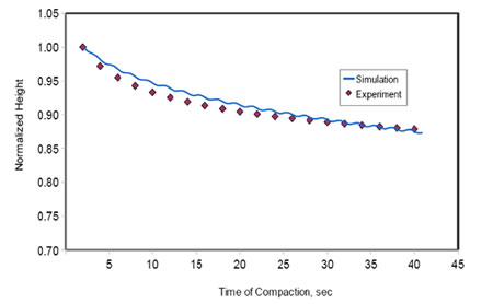
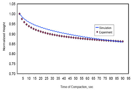
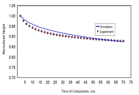
Mixtures from various projects were compacted using two angles of gyration, 1.25 and 2.0 degrees, to correspond to field compaction. The compaction curves at 1.25 degrees were used to determine the model's parameters, while the curves at an angle of 2.0 degrees were used to verify the ability of the model to fit experimental measurements different from those used to determine the parameters. Each of the compaction curves was divided into three parts: (1) time of compaction less than 15 s, (2) time of compaction between 15 and 30 s, and (3) time of compaction more than 30 s. The first part was used to estimate the parameters λ2 and ![]() of the viscosity function. The second part was used to estimate q2, and the third part was used to determine the parameters
of the viscosity function. The second part was used to estimate q2, and the third part was used to determine the parameters ![]() and n1 of the modulus function. The initial estimates were then slightly adjusted to minimize the difference between the model's results and the data of the whole compaction curve. The final simulation results using the parameters in table 3 are shown in figure 51 through figure 55 for an angle of 1.25 degrees and in figure 56 through figure 60 for an angle of 2.0 degrees. The results show that the model has a reasonable representation of the compaction curves at both angles. The nonsmooth response characteristics of the simulation, as can be observed from the plots, are a natural consequence of the boundary conditions and the fact that the calculations are made at an integration point in the material mesh that is at a slightly eccentric position from the axis of symmetry of the model.
and n1 of the modulus function. The initial estimates were then slightly adjusted to minimize the difference between the model's results and the data of the whole compaction curve. The final simulation results using the parameters in table 3 are shown in figure 51 through figure 55 for an angle of 1.25 degrees and in figure 56 through figure 60 for an angle of 2.0 degrees. The results show that the model has a reasonable representation of the compaction curves at both angles. The nonsmooth response characteristics of the simulation, as can be observed from the plots, are a natural consequence of the boundary conditions and the fact that the calculations are made at an integration point in the material mesh that is at a slightly eccentric position from the axis of symmetry of the model.
Table 3. Model parameters obtained from compaction data.
Mix Projects |
|
n1 |
|
λ2 |
q2 |
|---|---|---|---|---|---|
IH-35 |
2,000 |
5 |
1,400 |
0.25 |
−27 |
SH-36 |
2,400 |
4 |
1,800 |
0.22 |
−28 |
US-87 |
2,600 |
5 |
2,100 |
0.26 |
−27 |
US-259 |
2,400 |
5 |
1,700 |
0.21 |
−28 |
SH-21 |
2,500 |
4 |
2,000 |
0.22 |
−30 |
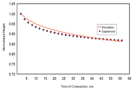
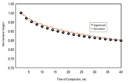
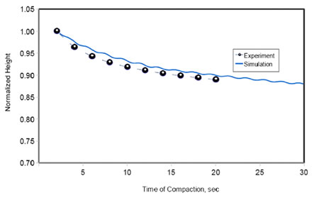
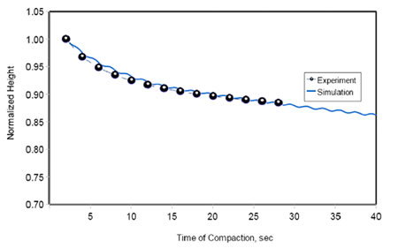
Figure 51. Chart. Fitting of the compaction data at 1.25 degrees for project IH-35.
Figure 52. Chart. Fitting of the compaction data at 1.25 degrees for project US-259.
Figure 53. Chart. Fitting of the compaction data at 1.25 degrees for project SH-36.
Figure 54. Chart. Fitting of the compaction data at 1.25 degrees for project SH-21.
Figure 55. Chart. Fitting of the compaction data at 1.25 degrees for project US-87.
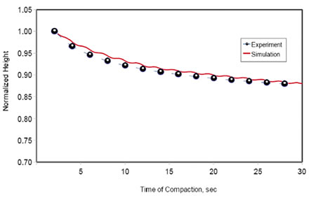
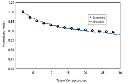
Figure 56. Chart. Prediction of the compaction data at 2.0 degrees for project IH-35.
Figure 57. Chart. Prediction of the compaction data at 2.0 degrees for project US-259.
Figure 58. Chart. Prediction of the compaction data at 2.0 degrees for project SH-36.
Figure 59. Chart. Prediction of the compaction data at 2.0 degrees for project SH-21.
Figure 60. Chart. Prediction of the compaction data at 2.0 degrees for project US-87.
The comparison between the parameters in table 3 and the mixture characteristics did not reveal clear and simple relationships. This could be attributed to the fact that each of the parameters, whether part of the modulus or viscosity function, is related to combinations of the mixture characteristics. The determination of these relationships requires the analysis of parameters of more mixtures in order to develop regression equations between the model's parameters and mixture characteristics. Nevertheless, there are some trends supporting the idea that relationships exist between material properties and model parameters. For example, the lowest values of ![]() and
and ![]() are for the stone matrix asphalt mixture in IH-35. These low values suggest better compactability, which could be attributed to the high asphalt content of this mixture. Also, the model results for very low angles of compaction do not agree well with what can be observed in the laboratory at such angles. This is because of the high compressibility built into the model to simulate the large deformations generally observed during compaction, which is not exhibited by actual mixes at very low angles of gyration.
are for the stone matrix asphalt mixture in IH-35. These low values suggest better compactability, which could be attributed to the high asphalt content of this mixture. Also, the model results for very low angles of compaction do not agree well with what can be observed in the laboratory at such angles. This is because of the high compressibility built into the model to simulate the large deformations generally observed during compaction, which is not exhibited by actual mixes at very low angles of gyration.
The parametric analysis conducted in this study showed that the compaction process is insensitive to changes in some of the model's parameters. Therefore, constant values were used for these parameters during all the FE simulations in order to simplify the process of finding the values of the remaining parameters. The parametric analysis demonstrated that some of the model's parameters are related mostly to the initial stage of compaction when the material exhibits low viscosity fluidlike behavior, while some parameters are related to the behavior of the mixture after it starts to exhibit a highly viscous fluid behavior and compaction rate decreases. A systematic method was developed to determine the model's parameters from the SGC curves. It was necessary to develop this method due to the difficulty of conducting conventional tests (e.g., triaxial or shear tests) to determine the model's parameters given the high compaction temperatures. The FE simulations demonstrated the capability of the constitutive model to simulate the SGC process at different compaction angles.