U.S. Department of Transportation
Federal Highway Administration
1200 New Jersey Avenue, SE
Washington, DC 20590
202-366-4000
Federal Highway Administration Research and Technology
Coordinating, Developing, and Delivering Highway Transportation Innovations
 |
| This report is an archived publication and may contain dated technical, contact, and link information |
|
Publication Number: FHWA-HRT-10-065 Date: December 2010 |
The purpose of a sensitivity analysis is to correlate various features of the output of the mathematical model to the different input factors and parameters of the model. The sensitivity analysis is constrained by a lack of experimental evidence for the mechanical response of HMA while compaction is being performed in the field. In order to establish a reference material response and aid in the sensitivity study, a reference parameter set was chosen. Since compaction of HMA manifests primarily in the volumetric changes that occur during the process, this study is based on a volumetric measure that quantifies material response. A comparison of the general volumetric viscous evolution response of the material (measured through the mathematical invariant det(G)-1 that represents the volumetric change in the viscous evolution tensor G) and its response when using a reference set of material parameters is presented.
The sensitivity analysis provides a general qualitative understanding of the trends of the material behavior in relation to the variation in parameters. The viscous evolution of the model as the parameters are varied is presented in figure 95 and figure 96. The model parameters used to study sensitivity are presented in table 8.
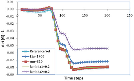
Figure 95. Chart. Evolution of the volumetric viscous gradient with a change in values of individual parameters ![]() ,
, ![]() , λ1, and λ2.
, λ1, and λ2.
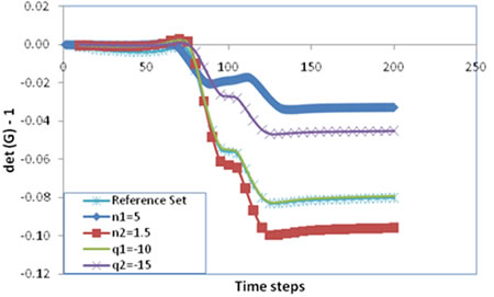
Figure 96. Chart. Evolution of the volumetric viscous gradient with a change in values of individual parameters n1, n2, q1, and q2.
Table 8. Parameters employed for the sensitivity study of the material.
Mix Parameter Sets |
|
n1 |
λ1 |
q1 |
|
n2 |
λ2 |
q2 |
|---|---|---|---|---|---|---|---|---|
Reference set |
620 |
4.0 |
0.25 |
−15 |
1,400 |
2.5 |
0.25 |
−20 |
Set 1 (change |
620 |
4.0 |
0.25 |
−15 |
1,700 |
2.5 |
0.25 |
−20 |
Set 2 (change |
810 |
4.0 |
0.25 |
−15 |
1,400 |
2.5 |
0.25 |
−20 |
Set 3 (change λ1) |
620 |
4.0 |
0.20 |
−15 |
1,400 |
2.5 |
0.25 |
−20 |
Set 4 (change λ2) |
620 |
4.0 |
0.25 |
−15 |
1,400 |
2.5 |
0.2 |
−20 |
Set 5 (change n1) |
620 |
3.0 |
0.25 |
−15 |
1,400 |
2.5 |
0.25 |
−20 |
Set 6 (change n2) |
620 |
4.0 |
0.25 |
−15 |
1,400 |
1.5 |
0.25 |
−20 |
Set 7 (change q1) |
620 |
4.0 |
0.25 |
−10 |
1,400 |
2.5 |
0.25 |
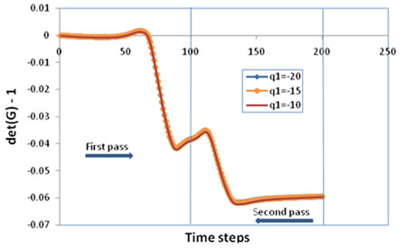
−20 |
Set 8 (change q2) |
620 |
4.0 |
0.25 |
−15 |
1,400 |
2.5 |
0.25 |
−15 |
Observations from the Sensitivity Analysis
The response of the material is stiffer (see figure 95) as the viscosity parameter ![]() is increased. This correlates to the response observed in the SGC simulations and is understood to be due to the material becoming a more viscous fluid as compaction progresses.
is increased. This correlates to the response observed in the SGC simulations and is understood to be due to the material becoming a more viscous fluid as compaction progresses.
The shear-modulus parameter ![]() causes a significant stiffening of the material in the initial stages of compaction. This can be observed in the response of the material in the first 50 time steps of the simulation. The comparative increase in the elastic rebound experienced by the mix in the initial stages, as
causes a significant stiffening of the material in the initial stages of compaction. This can be observed in the response of the material in the first 50 time steps of the simulation. The comparative increase in the elastic rebound experienced by the mix in the initial stages, as ![]() increases, corresponds to the constitutive assumption that the stored energy
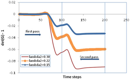
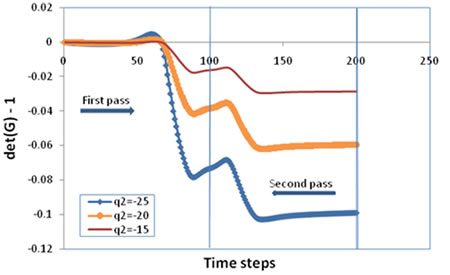
in the material is dependent on the shear-modulus function. Thus, as in the SGC simulations, the shear modulus affects the material response, but the viscous nature of the material dominates the response as the load traverses the pavement surface. A decrease in the λ1 and λ2 values also serves to make the material stiffer. λ1 has an effect on the model response only at the very beginning of compaction. Even at the initial stages, the influence of λ2 is just as significant, thereby drawing attention to the response through all compaction stages. After the initial stages, the response to changes in λ2 is dominant, as is the case in SGC compaction. As shown in figure 97, the regions of the parameters influence the gyratory compaction. This observation is useful for drawing generalized correlations between the material response expected in SGC compaction modeling and that expected in field compaction using the present model. As shown in figure 95, the increase in q2 results in the pavement responding significantly differently than when q1 is increased individually. This points toward q2 being the control parameter in a nonlinear transition of the material from the initially loose mix in the forward pass to a stiffer mix in the return pass. The lesser the magnitude of q2, the less permanent compaction is achieved. The pavement exhibits a relaxation mechanism as shown in figure 95 and figure 96. Note that the material is again compacted on the return pass, midway through the total number of time steps.
increases, corresponds to the constitutive assumption that the stored energy
in the material is dependent on the shear-modulus function. Thus, as in the SGC simulations, the shear modulus affects the material response, but the viscous nature of the material dominates the response as the load traverses the pavement surface. A decrease in the λ1 and λ2 values also serves to make the material stiffer. λ1 has an effect on the model response only at the very beginning of compaction. Even at the initial stages, the influence of λ2 is just as significant, thereby drawing attention to the response through all compaction stages. After the initial stages, the response to changes in λ2 is dominant, as is the case in SGC compaction. As shown in figure 97, the regions of the parameters influence the gyratory compaction. This observation is useful for drawing generalized correlations between the material response expected in SGC compaction modeling and that expected in field compaction using the present model. As shown in figure 95, the increase in q2 results in the pavement responding significantly differently than when q1 is increased individually. This points toward q2 being the control parameter in a nonlinear transition of the material from the initially loose mix in the forward pass to a stiffer mix in the return pass. The lesser the magnitude of q2, the less permanent compaction is achieved. The pavement exhibits a relaxation mechanism as shown in figure 95 and figure 96. Note that the material is again compacted on the return pass, midway through the total number of time steps.
Figure 97. Chart. Regions of influence of model parameters in gyratory compaction.(51)
The parametric analysis focused on the influence the parameters found not to affect the SGC curves (λ1, q1, and n2) had on field compaction. These results are presented in figure 98 through figure 103 by plotting the viscous deformation parameter (det(G)-1) for different model parameters.
Figure 98. Chart. Evolution of the volumetric viscous gradient with a change in λ1.
Figure 99. Chart. Evolution of the volumetric viscous gradient with a change in q1.
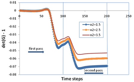
Figure 100. Chart. Evolution of the volumetric viscous gradient with a change in n2.
Figure 101. Chart. Evolution of the volumetric viscous gradient with a change in λ2.
Figure 102. Chart. Evolution of the volumetric viscous gradient with a change in q2.
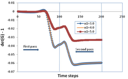
Figure 103. Chart. Evolution of the volumetric viscous gradient with a change in n1.
Correlation with Laboratory Compaction
Researchers sought to draw correlations between the behavior of model parameters during the SGC simulation and their behavior during the simulation of field compaction. The results were as follows:
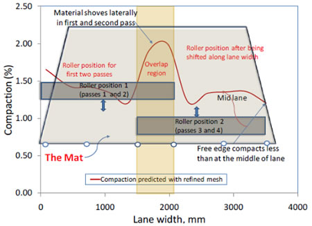
Asphalt pavements close to longitudinal joints tend to be compacted less than the center of the pavements. This is due to the tendency to apply fewer passes at the joints. The low confinement at some types of joints (unrestricted or unconfined joints) and the higher rate at which the mixture at the joint loses heat reduce the efficiency of compaction at the joint compared with the pavement center. Here, the compaction of longitudinal joints is studied by simulating the process using the model developed in finite elements. FE simulations were conducted to study the effects of longitudinal joints. Figure 63 shows the boundary conditions that are to be applied on the edges that have been fixed and on the edges that have been unrestrained, along with the longitudinal joints of the pavement. The model predicts a higher level of compaction close to the fixed edge of a lane (0.5 ft (0.1525 m)). The compaction predicted at the outer part of the lane, close to the unconfined/free edge (0.5 ft (0.1525 m)), is significantly lower because of the lack of a confining pressure close to the edge. The overlap zone between two roller passes contains the longitudinal joint where material shoving occurs to accommodate the compaction of the material. This kind of behavior is also observed in the field and is depicted in figure 104.
Figure 104. Chart. Plot representing the final compacted state of the material along the width of the pavement.
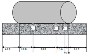
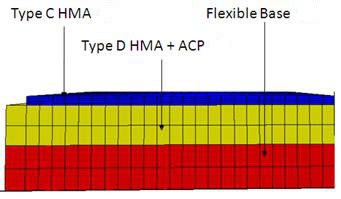
A section of highway SH-21 was compacted using a vibratory roller compactor to provide data for preliminary evaluation of the model developed in this study. The compactor had two steel drums with a width of 7 ft (2.135 m) and a distance of 12 ft (3.66 m) between the centers of the drums. The total weight of the roller was 27,783 lb (12,613 kg); the front drum had a weight of 13,980 lb (6,347 kg), and the back drum had a weight of 13,803 lb (6,266 kg). The roller was operated in vibration mode with about 3,000 vibrations per minute at a speed of 2 to 3 mi/h (3.2 to 4.8 km/h). Aggregate characteristics (angularity, texture, and sphericity) were measured using the Aggregate Imaging System. Higher numbers for angularity and texture indices mean higher aggregate angularity and texture. Higher sphericity values indicate that particles are less flat and elongated (a sphere has a value of 1). The properties of the various layers are shown in table 9.
Table 9. Material properties used for the SH-21 project.
Layer |
Modulus, psi |
Poisson Ratio, n |
|---|---|---|
2.0-inch Type C HMA |
Refer to table 10 |
|
2.0-inch of Type D HMA |
450,000 |
0.30 |
18.0-inch flexible (granular) base |
30,000 |
0.35 |
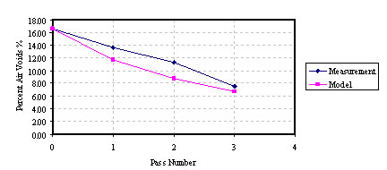
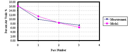
The FE model was used to simulate field rolling compaction on material 12-ft (3.66-m) wide with the roller centered on the material, as shown in figure 105. The initial simulations were conducted using the material model parameters from SGC simulations, shown in table 10. However, the percent of compaction was much lower than the experimental measurements in terms of percent air void (%AV). Computations of percent compaction close to field air voids were obtained only by reducing the viscosity coefficient ![]() to a value less than 72.51 ksi·s (500 MPa·s). The results shown in figure 106 are for
to a value less than 72.51 ksi·s (500 MPa·s). The results shown in figure 106 are for ![]() of 29 ksi·s (200 MPa·s). The laboratory compaction curves were described well using a
of 29 ksi·s (200 MPa·s). The laboratory compaction curves were described well using a ![]() value of 290.07 ksi·s (2000 MPa·s), as shown in table 10.
value of 290.07 ksi·s (2000 MPa·s), as shown in table 10.
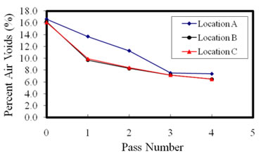
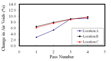
The measured %AV is shown in figure 106, and the change in %AV is shown in figure 107. A comparison of the typical simulated responses using the FE model shows that the model developed predicts a trend of compaction over multiple passes similar to trends measured in the field (see figure 108 through figure 110).
Figure 105. Illustration. Schematic of a roller on a material with three locations for density measurements.(49)
Table 10. Model parameters used for projects SH-21, US-87, and US-259..
Highway Projects |
Parameter Sets |
|
n1 |
λ1 |
q1 |
|
n2 |
λ2 |
q2 |
|---|---|---|---|---|---|---|---|---|---|
SH-21 |
SGC |
2,500 |
4 |
0.25 |
−25 |
2,000 |
2.5 |
0.22 |
−30 |
Field |
2,500 |
4 |
0.25 |
−25 |
2,00 |
2.5 |
0.22 |
−30 |
|
US-87 |
SGC |
2,600 |
5 |
0.25 |
−25 |
2,100 |
2.5 |
0.26 |
−27 |
Field |
2,300 |
5 |
0.25 |
−25 |
2,100 |
2.5 |
0.26 |
−27 |
|
US-259 |
SGC |
2,400 |
5 |
0.25 |
−25 |
1,700 |
2.5 |
0.21 |
−28 |
Field |
2,150 |
5 |
0.25 |
−25 |
1,700 |
2.5 |
0.21 |
−28 |
Figure 106. Chart. Measurements of the %AV in the asphalt mix.(49)
Figure 107. Chart. Measurements of change in %AV in the asphalt mix.(49)
Figure 108. Chart. Measurements and modeling results of %AV at point A of the pavement locations shown in figure 105.
Figure 109. Chart. Measurements and modeling results of %AV at point B of the pavement locations shown in figure 105.
Figure 110. Chart. Measurements and modeling results of %AV at point C of the pavement locations shown in figure 105.
The difference between the simulation parameters obtained from the laboratory and field compaction processes raises important points regarding the modeling aspects that need to be addressed to accurately describe both processes. One aspect is the accuracy of representing the boundary and loading conditions of the laboratory and the field. For example, the load used in simulating field compaction is quasi-static and does not accurately represent the actual dynamic forces applied by a vibratory roller. There is also the mathematically and computationally complex contact problem between the roller drum and the asphalt pavement surface that is not addressed in the FE simulations.
Another important cause of the differences in the model's parameters is the material model's limited ability to represent the various mechanisms involved in the laboratory and field compaction processes. This cause is less obvious and harder to address compared with the differences in boundary conditions. For example, the asphalt mix behavior is rate dependent, but the model might be limited in capturing the rate dependency. This rate dependency would not significantly affect the SGC simulations because the compaction is conducted under continuous application of one loading rate of 30 revolutions per minute. Such a limitation, however, would be clearly manifested in field simulations because the rate of loading could vary considerably. Consequently, calibration with field compaction data would be required as the field conditions could vary beyond the laboratory experiments used to determine the model's parameters.
In order to further examine the utility of the model in simulating field compaction trends, field rolling compaction was simulated to match the rolling patterns in two highway projects, a US-87 paving job near Port Lavaca in Calhoun County, TX, in October 2006 and a section of US-259 located in Rusk County, TX, in February 2007.(7) Specimens from both projects were obtained from the wheel path, between the wheel path, and on the longitudinal joint (restrained and unrestrained). The asphalt mixtures and compaction data were part of a study funded by the Texas Department of Transportation to evaluate the influence of various field compaction methods on asphalt-mixture properties. The properties of the top asphalt mixture are reported in table 11 and table 12.
Table 11. Summary of mixture designs..
Highway Project |
Mixture Type |
Aggregate Type |
Binder Grade |
AC (Percent) |
Gmm |
VMA |
Design |
|---|---|---|---|---|---|---|---|
SH-21 |
Type C |
Limestone |
PG 70-22 |
4.7 |
2.467 |
14.3 |
3.0 |
US-87 |
Type C |
Siliceous River Gravel |
PG 76-22S |
4.3 |
2.439 |
13.8 |
4.0 |
US-259 |
Type C |
Sandstone and Limestone |
PG 70-22S |
4.3 |
2.478 |
13.1 |
3.0 |
Table 12. Summary of properties of mixture constituents..
Highway Project |
Binder Viscosity, |
Aggregate Texture Index |
Aggregate Angularity Index |
Aggregate Sphericity |
|---|---|---|---|---|
SH-21 |
0.883 |
106 |
2,811 |
0.708 |
US-87 |
2.258 |
112 |
3,062 |
0.651 |
US-259 |
0.818 |
189 |
2,791 |
0.618 |
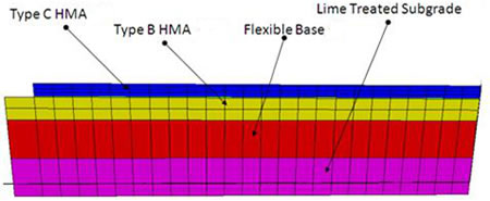
US-87 is a four-lane divided highway. Test sections were located on the northbound outside lane. The mixture was Type C (Texas Department of Transportation 1993 specification) designed with Fordyce Gravel and Colorado Materials limestone screening with 4.3 percent PG 76-22S binder. The Type C mixture is similar to the coarse-graded Superpave® mixture. The Type C mixture was laid on a Type B material, which primarily included crushed river gravel. The thickness of the Type C layer was 2 inches (50 mm). The mixture was laid with a 16 ft (4.8 m) material width, with 1.5 ft (4.5 m) tapered on one side. The structure of the pavement for the US-87 pavement project is presented in figure 111, the layer properties are given in table 13, and the width of the top layer of material is shown in figure 112.
Figure 111. Illustration. Pavement structure for the US-87 project.
Table 13. Material properties used for the US-87 project..
Layer |
Modulus, psi |
Poisson Ratio, n |
|---|---|---|
2.0-inch Type C HMA |
Refer to table 10 |
|
3.5-inch Type B HMA |
450,000 |
0.30 |
6.0-inch flexible (granular) base |
30,000 |
0.35 |
6.0-inch lime-treated subgrade |
12,000 |
0.45 |
Figure 112. Chart. Schematic for the rolling patterns for the US-87 project.
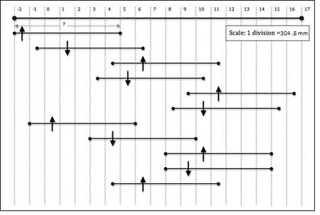
The general rolling pattern can be described as breakdown by a steel-wheel vibratory roller and pneumatic wheel roller for both intermediate and finish rolling. In addition, the rolling pattern consisted of progressively moving the vibratory steel-wheel roller in transverse directions, with the pneumatic wheel roller again acting as both the intermediate and finish roller. The sequence and locations of the roller are simulated approximately, along with the boundary conditions representative of the restrained and unrestrained edges of the pavement, and are indicated by the bars in the schematic in figure 112. In the schematic, the inner edge of a lane is indicated by the vertical dotted line passing through 0. The roller locations are represented with respect to this line as the datum to measure distance. The line segments represent rollers with their rolling directions. An upward arrow indicates forward rolling, and a downward arrow indicates the reverse. The rolling pattern and the measured %AV are presented in table 14. There were 11 total passes in the compaction process involving the vibratory roller, with 9 passes in vibratory mode and 2 passes in static mode.
Table 14. Rolling pattern and %AV measured in the field for the US-87 project..
Core Group |
Distance from Edge (ft) |
Vibratory Mode |
Static Mode |
%AV |
|---|---|---|---|---|
1 |
1 |
3 |
1 |
9.65 |
2 |
4 |
5 |
1 |
6.77 |
3 |
7 |
3 |
1 |
7.33 |
4 |
10 |
6 |
2 |
5.01 |
The overlay in the US-259 project used a Type C surface mixture compacted in a 2-inch (5-cm) lift thickness. The coarse part of the aggregate was sandstone, and the intermediate- and fine-size particles were limestone. The mix had 11 percent field sand and 4.3 percent PG 70 22S binder. The test sections were in the southbound outside lane. Type C mix was laid on top of a recently compacted Type D level-up course where the Type D mixture was similar to a Superpave® fine graded mixture. The paving width was approximately 15 ft (4.57 m) (including shoulder), and a vertical longitudinal joint was maintained. The structure of the pavement for the US-259 pavement project is presented in figure 113, the layer properties are given in table 15, and the width of the top layer of material is shown in figure 114.
Figure 113. Illustration. Pavement structure for the US-259 project.
Table 15. Material properties used for the US-259 project..
Layer |
Modulus, psi |
Poisson Ratio, n |
|---|---|---|
2.0-inch Type C HMA |
Refer to table 10 |
|
1.25-inch Type D HMA |
450,000 |
0.30 |
7- to 8-inch asphalt concrete pavement |
400,000 |
0.30 |
10-inch flexible (granular) base |
34,000 |
0.35 |
Figure 114. Chart. Schematic for the rolling patterns for the US-259 project.
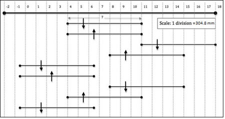
The general rolling pattern can be described as breakdown by a steel-wheel vibratory roller and pneumatic wheel roller for both intermediate and finish rolling. In addition, the rolling pattern consisted of progressively moving the vibratory steel-wheel roller in transverse directions, with the pneumatic wheel roller acting as both the intermediate and finish roller. The sequence and locations of the roller are simulated approximately, along with the boundary conditions representative of the restrained and unrestrained edges of the pavement, and are indicated by the bars in the schematic in figure 114. In the schematic, the inner edge of a lane is indicated by the vertical dotted line passing through 0. The roller locations are represented with respect to this line as the datum to measure distance. The line segments represent rollers with their rolling directions. The rolling patterns and the %AV are presented in table 16. There were nine total passes in the compaction process involving the vibratory roller, with five passes in vibratory mode and four in static mode.
Table 16. Rolling pattern and %AV measured in the field for the US-259 project..
Core Group |
Distance from Edge (ft) |
Vibratory Mode |
Static Mode |
%AV |
|---|---|---|---|---|
1 |
1 |
1 |
2 |
11.26 |
2 |
5 |
3 |
3 |
7.70 |
3 |
8 |
3 |
2 |
8.12 |
4 |
11 |
2 |
2 |
10.78 |
5 |
14 |
2 |
1 |
9.27 |
Observations from Field Compaction Simulations for US-87 and US-259
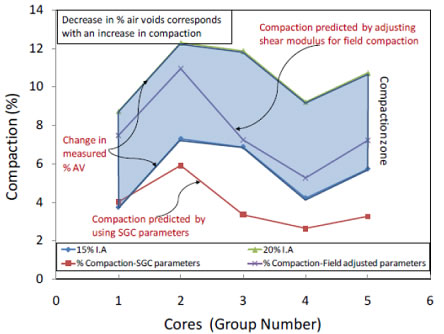
As in actual field compaction, the initial air voids generally vary between 15 and 20 percent of the volume of the mix, and the measured %AV is adjusted by using these two initial air void values to calculate the change in measured %AV, which is more indicative of the compaction the material has experienced. The change in measured %AV is then compared directly to the percent-compaction values predicted by the FE model (see table 17 and table 18). A compaction zone is enclosed by the use of two initial %AV values, as indicated in figure 115 and figure 116, where the measured and calculated percent compaction at different locations across the material are compared at the end of rolling pattern cycles. In the figures, the comparisons are made per core group, which represents different locations across the material relative to the edge (see table 9 through table 16).
Table 17. Change in measured %AV in the field and calculated percent compaction for the US-87 project..
Core Group |
15 Percent Initial |
20 Percent Initial |
Compaction Using SGC Parameters (Percent) |
Compaction Using Field Parameters (Percent) |
|---|---|---|---|---|
1 |
5.35 |
10.35 |
3.52 |
7.50 |
2 |
8.23 |
13.23 |
5.17 |
10.39 |
3 |
7.67 |
12.67 |
4.42 |
9.49 |
4 |
9.99 |
14.99 |
6.04 |
12.83 |
Table 18. Change in measured %AV in the field and calculated percent compaction for the US-259 project..
Core Group |
15 Percent Initial |
20 Percent Initial |
Compaction Using SGC Parameters (Percent) |
Compaction Using Field Parameters (Percent) |
|---|---|---|---|---|
1 |
3.74 |
8.74 |
4.02 |
7.48 |
2 |
7.30 |
12.30 |
5.92 |
10.95 |
3 |
6.88 |
11.88 |
3.36 |
7.25 |
4 |
4.22 |
9.22 |
2.64 |
5.28 |
5 |
5.73 |
10.73 |
3.26 |
7.22 |
Figure 115. Chart. Comparison of the total percent compaction from simulations with the general trend of the %AV measured at the end of the field compaction process for US-87.
Figure 116. Chart. Total percent compaction from simulations compared to the general trend of the %AV measured at the end of the field compaction process for US-259.
The percent-compaction values were calculated using parameters from SGC compaction of these two mixes as well as field-adjusted parameters. The compaction predicted by the SGC parameters was outside the range of the change in %AV measured in the field (see figure 115 and figure 116). Therefore, the parameters were adjusted so that the compaction obtained in simulations was contained within the range of measured %AV values. The parameters used for simulation purposes are shown in table 10. As shown in figure 115 and figure 116, within the compaction zone the behavior of the mix in the simulations correlates well with the trends observed in the field. The type of compaction in each project (based on the combination of the type of roller and the rolling pattern) correlates directly to the measured change in %AV for the corresponding core groups (see table 17 and table 18). The greater the measured change in %AV, the more compaction occurs at that location. This behavior is reflected in figure 115 and figure 116 for simulations of both projects and, in that sense, agrees with reality.
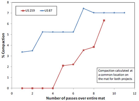
The simulation model is capable of providing further insight into field compaction trends when using the measured %AV to gauge material response. As can be seen in figure 117 (comparing the response of two materials at the same location relative to the edge of the material), the simulations predict that the US-87 material will undergo more compaction by the end of the whole process than the US-259 material. This is in direct correlation to the higher change in measured %AV for the US-87 pavement (table 17, core group 1) as compared to the change in measured %AV for the US-259 pavement (table 18, core group 1).
Figure 117. Chart. Comparison of prediction of percent compaction per roller pass for US-87 and US-259.
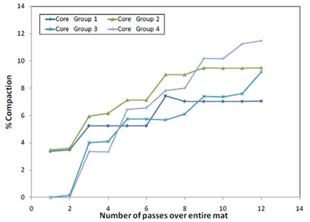
Some interesting observations can be drawn from the response of the material as it is subject to different roller passes. From figure 118 (with the roller patterns from table 14), the following observations of the material behavior of US-87 pavement undergoing compaction can be made:
Figure 118. Chart. Prediction of percent compaction per roller pass across the material for US-87 (cores taken at four locations).
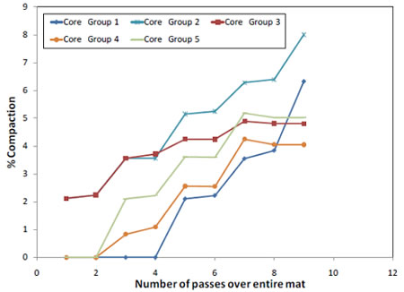
From figure 119, the following observations for the compaction response of the pavement material for US-259 can be made:
Figure 119. Chart. Prediction of percent compaction per roller pass across the material for US-259 (cores taken at four locations).
In conclusion, researchers observed that compaction simulated across the pavement over the different roller passes correlates with the compaction measured (through a change in %AV) in the field. The compaction simulation using model parameters from the SGC simulations is similar to the measured values. These parameters, with a simple shift in one of the parameter values (![]() ), can therefore be used to predict field compaction, allowing a correlation between laboratory and field compaction simulations. A compaction-zone characteristic of each mix type can be predicted. Applying vibratory-mode loads initially causes a more uniform compaction (in terms of the percent compaction per pass). Rolling patterns and load locations are of utmost importance in determining the amount and type of compaction (more uniform or less uniform). The simulation model provides an opportunity to experiment with different rolling patterns to achieve a specific percent compaction or a certain trend in the uniformity of compaction from pass to pass. Considerable variability exists in the compaction trends. This has been shown through the study of two projects. The variability in trends due to loading patterns is a natural reflection of the nonlinear nature of the materials employed. Only vibratory and static wheel loads have been considered. Simulation of finish rolling through use of pneumatic rollers was not considered.
), can therefore be used to predict field compaction, allowing a correlation between laboratory and field compaction simulations. A compaction-zone characteristic of each mix type can be predicted. Applying vibratory-mode loads initially causes a more uniform compaction (in terms of the percent compaction per pass). Rolling patterns and load locations are of utmost importance in determining the amount and type of compaction (more uniform or less uniform). The simulation model provides an opportunity to experiment with different rolling patterns to achieve a specific percent compaction or a certain trend in the uniformity of compaction from pass to pass. Considerable variability exists in the compaction trends. This has been shown through the study of two projects. The variability in trends due to loading patterns is a natural reflection of the nonlinear nature of the materials employed. Only vibratory and static wheel loads have been considered. Simulation of finish rolling through use of pneumatic rollers was not considered.