Modeling of Hot-Mix Asphalt Compaction: A Thermodynamics-Based Compressible Viscoelastic Model

CHAPTER 6. FE SIMULATION OF FIELD COMPACTION

INTRODUCTION

Development of a useful simulation environment to study field compaction of HMA provides a unique challenge because of the complex physical interactions involved. A framework composed of a nonlinear material model coupled with an advanced numerical simulation environment (CAPA 3D) was chosen for this study. The theoretical model employed for the FE model development was adapted from the HMA material model presented in Koneru et al.⁽⁴⁸⁾ This model was subsequently utilized for the simulation of the compaction mechanism of the SGC. The results of the study have been documented in Masad et al.⁽⁴⁹⁾ Here, the chosen numerical framework is used to extend the work presented in Koneru et al. and Masad et al. to specifically study the material model's behavior when subject to the conditions pertinent to field compaction of HMA.^(48,49)

The simulation of the rolling compaction process includes many challenges in terms of representing the complex physical interactions in a numerical model. Some of the chief factors that influence the research related to the field compaction simulation are as follows:

• Development of a contact-area-determining algorithm was needed to determine the effective area of a given FE mesh in contact with a roller used for applying a compacting load on the material. Since the material model chosen from Koneru et al. was a compressible viscoelastic material, devising an algorithm for contact had to be considered carefully.⁽⁴⁸⁾
• Because of the large variation in the material properties of the different layers of a pavement structure, it was anticipated that numerically simulating the interactions of the layers would require specialized techniques. For this purpose, researchers used specialized finite elements for resolving the interfacial contact issues.
• Because of the application of a load that is translated over the surface in field compaction, special care was taken to avoid wave reflections from boundaries and interfaces. Such interference waves produced within the material can affect the solution in a numerical experiment. A standard technique to deal with such detrimental effects is the use of "impedance layers" in FE meshes. (See Sluys for further details on the utility and development of such elements.)⁽⁵⁵⁾
• The effect of the stiffness of substructure layers needed to be studied because the structural response of any material is, in general, subject to the material it interacts with in response to external influences.
• A study of the sensitivity of compaction to model parameters provided an opportunity to understand the behavior of the model in a structural setting. The change in behavior of the FE model with changes in parameter values aids in the estimation of the model behavior based on given input conditions to the system. Because of the physical interactions involved and a lack of detailed experimental data, the researchers needed such a study to draw correlations between laboratory and field compaction activities.

FE MODEL

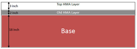
A typical pavement structure used for simulating field compaction is shown in figure 61. It consists of the following three layers: a base layer consisting of aggregate and/or soil approximately 18 inches (457.2 mm) thick, an overlay on top of the base layer consisting of old HMA approximately 2 inches (50.8 mm) thick, and a 3 inch (76.2 mm)-thick top layer of freshly laid HMA that will be compacted by rolling.

Figure 61. Illustration. Pavement structure typically employed for studying field compaction.

The general structure of CAPA-3D facilitates quick, flexible testing of material models and has been presented in detail by Scarpas.^(53,54) For the implementation of the chosen material model, two interface subroutines are input into CAPA-3D. The necessary model parameters, boundary conditions, and algorithmic logic necessary for the required stress updates at each material point are provided to CAPA-3D through user-interface files for each type of necessary data. The required stress update subroutine was devised from the equations obtained through a numerical discretization of the constitutive relations of the material model chosen. The stress-update subroutine consists of a system of nonlinear algebraic equations that are iteratively integrated at each material-integration point and each step in the time domain. The computational sequences devised are then provided as Fortran instructions that can be embedded directly into the CAPA 3D interface. Details on the usage of the computational system are provided by Scarpas.⁽⁵³⁾

FE Mesh Used for Simulation

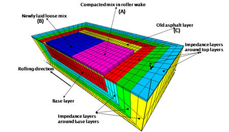
Some of the important characteristics of the FE mesh used for simulating compaction (shown in figure 62) are as follows:

• The representative mesh has material in three different layers along with the material already compacted by the roller. The mesh is a half-sectional view. The symmetry of boundary conditions sometimes allows the half mesh to be employed instead of the full mesh.
• The typical geometry of the mesh is given the typical thicknesses shown in figure 61, a lane width of 12 ft (3.66 m), and a total top-layer length in the direction of rolling of 44 inches (1,117.6 mm). The top layer consists of a newly laid mix and a previously compacted mix, each 22 inches (558.8 mm) in length in the direction of rolling.
• The typical material properties used for the three layers are given in table 4.
• All the finite elements used for the structural layers are 20-noded, solid, three-dimensional continuum elements. Details of other choices and options for the elements available for use in CAPA-3D are available from Scarpas.⁽⁵³⁾
• The interfacial contact between any pair of layers among the uncompacted HMA, the old HMA layer underneath, and the previously compacted layer on top is resolved through use of a special interface element available in CAPA-3D.⁽⁵³⁾ Use of this layer is strictly to preserve the contact between the layers, and hence, these special elements do not have any structural utility.
• Impedance layers surrounding the base layer and other such elements surrounding the top HMA and old HMA layers (as shown in figure 62) minimize the dynamic loading effects.
• The analyses are performed by fixing the time increments at 0.05 s. This value is based on the actual velocity of the roller and takes into account a need for consistent numerical stability of the algorithm. The time increments are calculated by first determining the total time per pass by dividing the total distance of travel (22 inches (558.8 mm)) by the speed of travel of the roller (initially set to 4.4 inches/s (111.76 mm/s)) and then multiplying by the total number of time steps desired per pass (assumed 100 here).

Figure 62. Illustration. Sectional view of the FE mesh used for setting up field compaction simulations.

Table 4. Typical material properties of pavement structural layers.

Boundary Conditions for Simulating Field Compaction

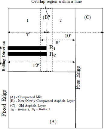
The boundary conditions most frequently utilized are presented in figure 63. The schematic illustrates that the fixed edge corresponds with the inner edge of the pavement lane while the free edge corresponds with the outer edge of the lane. The displacement on the fixed edge is thereby constrained in the lateral direction (z-coordinate direction for the given mesh orientation), the free edge is allowed to move unconstrained, and a traction-free boundary condition is employed.

When the middle lane of a highway is to be simulated, simplifying further requires assuming symmetry in boundary conditions and employing a half mesh along the direction of rolling. In this case, the half-sectional mesh represented in figure 62 is sufficient for the simulation.

Figure 63. Illustration. Schematic diagram illustrating the edges of the lane that correspond to fixed and free edges of the mesh in figure 62.

Response to Moving Load

This section discusses the typical response of the material to a moving load in field compaction. The simulations were performed with material parameters that correspond to those in table 5. The same set of parameters in SGC and field compactions do not provide the same level of volumetric reduction because of significantly different boundary conditions such as confinement, temperature changes, uniformity and nonuniformity of applied loads, etc.

Table 5. Parameters used to study the typical material response during field compaction.

1 MPa = 0.145 ksi

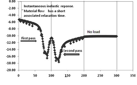
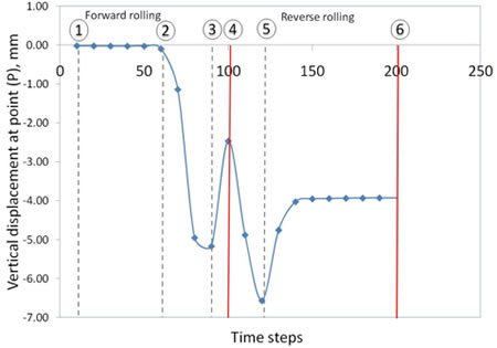
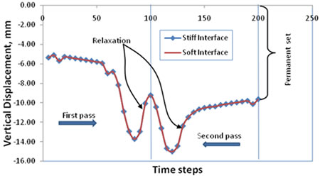
The typical response curve obtained from the simulations employing the previously described mesh subject to the specified boundary conditions is shown in figure 64. The response curve represents the compaction experienced at a point in the roller path as the roller passes over it and returns for a second pass from the opposite direction. The annotation arrows signify the forward motion in the first pass and the reverse-direction motion in the second pass. Finally, the load is removed and the material allowed to relax as much as possible. Thereafter, the material finally exhibits its state of permanent deformation, as seen in figure 64.

Figure 64. Chart. Typical displacement curve for a node under the cylindrical load for a cycle with forward and return passes followed by a forward pass with the load removed.

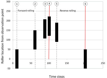
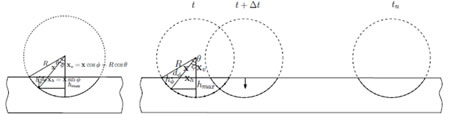
Figure 65 and figure 66 illustrate the relationship between the roller position with a contact area of 3.9 inches (100 mm) and the deflection experienced by a point P near the surface of the pavement. The illustrations are for a mixture that does not have instantaneous elastic response. Due to the viscoelastic nature of the material, the deflection at point P starts when the center of the roller has passed the point. The point continues to deform vertically as the roller moves forward.

When the roller is at point 4, the mixture at P rebounds some of its vertical deflection because it is out of the region of influence of the roller. Also, point 4 marks the time at which the roller starts to move back toward P. Further deflection occurs as the roller again approaches P (point 5). The final deflection is marked by point 6.

Figure 65. Chart. Vertical displacement observed at point P on the path of the roller.

Figure 66. Chart. Roller location from observation point P.

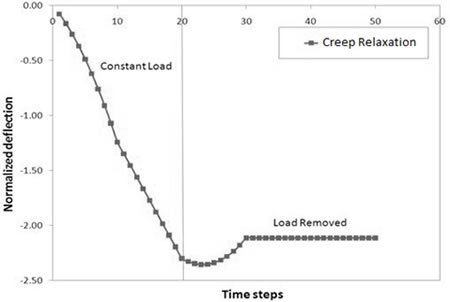
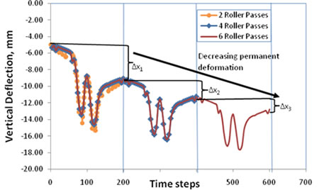
Each pass over the material results in permanent deformation upon unloading, as shown in figure 67. The deformation therefore builds up incrementally with each pass. However, as shown in figure 68, the increments decrease in magnitude due to material densification as the number of passes increases.

Figure 67. Chart. Deflection at the node of interest when a load is applied for a short duration and then removed.

Figure 68. Chart. Permanent deformation prediction of the model in multiple-pass loading.

Implementing a Contact-Area Algorithm

The objective was to implement an algorithm for load application on flexible pavement. Development of the new algorithm furthers the ability to simulate the compaction loading. The loading algorithm used in this project was based on translating a distributed load across the pavement.

The load was applied in the form of a grid of loading patches independent of the FE mesh. The pressure in each loading patch was uniform. By combining a suitable number of loading patches, any desired distribution of surface loads could be simulated. The loading patches were translated along the surface of the pavement to simulate the moving roller.

A process was developed for determining the pressure of each of the loading patches. The process involves the determination of the contact area between the roller and the pavement (see figure 69). A displacement that mimics the cylindrical profile of the roller is applied on the surface of the pavement. The number of nodes in the contact area is determined such that the summation of their nodal forces is equal to the weight of the roller (see figure 70). Different numbers of elements are maintained in contact to balance the dead weight of the roller.

Figure 69. Illustration. Roller contact geometry for static indentation and during motion.

Figure 70. Chart. Indentation of a cylindrical roller into pavement.

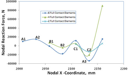
The plots presented in figure 71 represent the nodal reaction forces in the elements in response to the applied dead load of the roller as the contact area (represented by the number of elements in contact) is changed. A1 and A2 represent the edge and middle nodal forces of the same orientation in an element when considering six elements in contact between the roller and the material. Similarly, B1 and B2 represent the respective nodal forces at the edge and middle nodes of an element when four elements are chosen in contact, and C1 and C2 are nodal forces when two elements are chosen in contact. On the basis of the nodal forces in the contact area, the pressure in each loading patch was determined according to FE procedures.⁽⁵⁶⁾

Figure 71. Chart. Change in nodal reaction forces as the load is applied over a smaller area.

Once the compaction load is determined, the load is translated over the pavement, providing a loading effect similar to sliding a roller over pavement. The exact mechanics to establish a rolling-type contact between the roller and the nonlinear pavement material require in-depth exploration of the field of nonlinear contact mechanics and has not yet been implemented in the FE model developed for this project.

The loading pattern was used to simulate the compaction of asphalt pavements with a roller travel speed of 3.0 mi/h (4.8 km/h). This speed is in the range of values typically used in the field and reported in table 6.

Table 6. Typical roller-speed ranges.⁽¹⁾

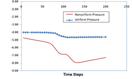
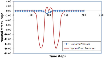
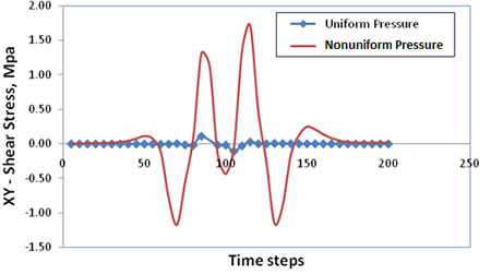
The plots in figure 72 though figure 74 are indicative of the differences observed in the displacement and stress response in an element in the direct path of the traversing load using the currently developed contact-area algorithm and the previously available loading algorithm in CAPA-3D, where the load is applied uniformly over all the finite elements in contact with the roller. The plots are representative of the response of the material at a node directly under the load (experiencing maximum normal distress) at the beginning of the simulation. The stress response of the pavement while the new cylinder indentation algorithm (nonuniform pressure) is employed is characteristic of the nonuniform stress reactions obtained in a 20-noded element, whereas the algorithm previously in use strictly enforced uniform pressure at all nodes under a loaded area at a given instant of time. This, therefore, validates the choice of the use of the cylinder indentation algorithm to better represent the physical contact situation between the roller and the pavement. The simulation results presented in this section utilize the model parameters for the SH-21 project simulations for the SGC (see Masad et al.)⁽⁴⁹⁾ The material parameters used for these comparisons are presented in table 7.

Figure 72. Chart. Comparison of vertical displacement for the two different patterns of loading.

Figure 73. Chart. Comparison of the normal stress distribution at the pavement's top surface due to different loading patterns.

Figure 74. Chart. Comparison of the shear-stress (XY) distribution of the pavement's top surface due to different loading patterns (on the plane of symmetry).

Table 7. Material parameters used to investigate the contact algorithm, interface effects, impedance element effects, and the effect of base stiffness.

1 MPa = 0.145 ksi

Normal Stresses Predicted by Model

The solution of a cylinder indented into an elastic medium (semi-infinite half space) was compared to the solution from the material model by balancing the self-weight of the roller with the normal reaction from the material. Then, the mean contact pressure used for the elastic solution was calculated using the equation in figure 75.

Figure 75. Equation. Mean contact pressure.

In this equation, P is the load per unit thickness in the z-direction, and a is the radius of contact. Here, the self-weight per unit of pavement width is used for P. The normal stress in the elastic medium is given by the equation in figure 76.

Figure 76. Equation. Normal stress in elastic medium.

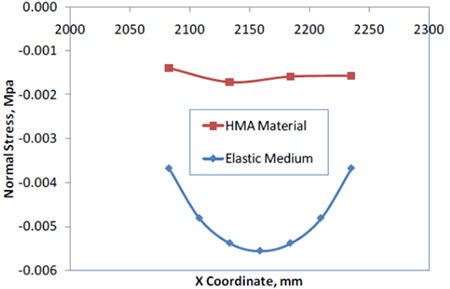
This representation of the solution indicates that the normal stress is expressed solely as a function of the position x and the mean contact pressure P_m. This relationship is illustrated in figure 77 in comparison to the instantaneous normal stress produced in the HMA material used in the compaction simulations with the same mean normal pressure applied. The comparatively higher stresses in the elastic medium at a given mean contact pressure are due to the lack of any dissipative mechanism in the elastic material. The model employed for representing the HMA develops dissipative responses in a nonlinear manner, and hence, the instantaneous response shows less stress. Also, the low level of stress in the HMA shows the low-viscosity fluidlike precompaction behavior of the model.

Figure 77. Chart. Comparison of the normal stress predicted by the model to the normal stress predicted for an elastic medium (for the same mean contact pressure, P_m).

Interface Elements

The FE analysis is dependent on the use of interface element layers between the top asphalt layer and the previously compacted asphalt layer as well as between the top newly laid asphalt and the old asphalt sublayer. This is due to the differences in properties of the loose mix and the stiff old asphalt layer. Hence, the specialized interface elements are employed to resolve the contact issues that arise due to the large variation in properties of material on either side of the interface. With the establishment and implementation of a useful contact-area algorithm in CAPA-3D, the analysis is performed to obtain insight into the effect of the interface elements. The use of interface elements provides a numerically stable and converging simulation. These interface elements do not contribute to the structural properties of the whole structure, and their applicability has been documented.⁽⁵⁴⁾ The interface elements to be used require the specification of two shear-stiffness and one normal-stiffness moduli. These stiffness values are used in the numerical algorithm to ensure contact is maintained between the layers by artificially attaching the corresponding nodes of the layers through a mathematical expression that governs their relative motion. The shear stiffness is used to govern the relative sliding of the layers, whereas the normal stiffness is used to prevent mesh penetration of the finite elements of a stiffer material into those of a soft material.

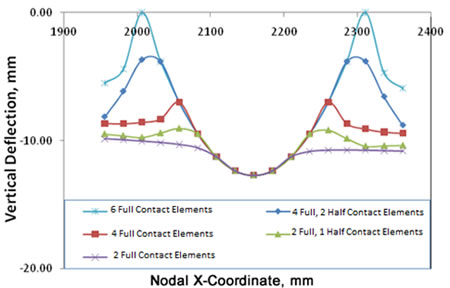
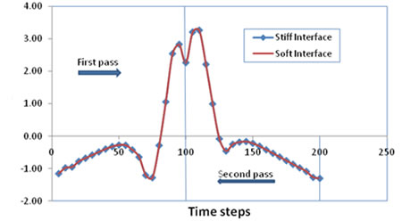
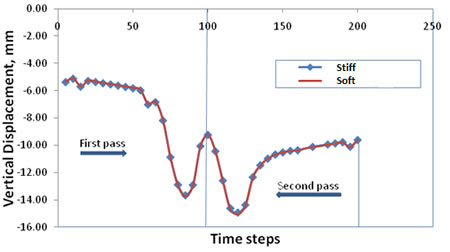
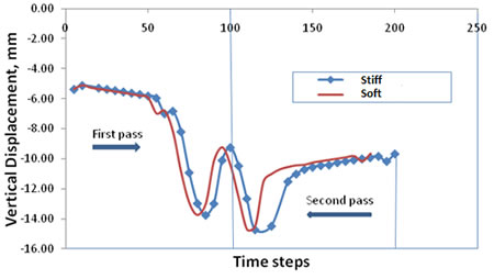
The results of FE analysis using the interface layer are presented in figure 78 through figure 81. The two shear-stiffness and one normal-stiffness properties are varied, and the resulting structural behavior of the HMA material is observed. The shear moduli are individually made stiffer, and a comparison is drawn to a reference set of interface-element stiffnesses. The same comparison is made after normal stress is made less stiff. It can be observed in figure 78 through figure 81 that the use of interface elements does not adversely affect the normal and in-plane displacement response of the model. The slight deviation observed when z-direction shear is stiffened is attributed to the structure of the mesh. The mesh used is longer in the z-direction, and hence, the effects of free boundaries are more pronounced. The situation is rectified by using a higher stiffness value because, beyond such a value, the interface exhibits similar behavior in the x-direction.

Figure 78. Chart. Comparison of pavement vertical response as the normal stiffness of the interface elements is lowered by an order of magnitude from 1,451 ksi (10,000 MPa) to 145 ksi (1,000 MPa).

Figure 79. Chart. Comparison of pavement response in the rolling direction as the normal stiffness of the interface elements is lowered by an order of magnitude from 1,450 ksi (10,000 MPa) to 145 ksi (1,000 MPa).

Figure 80. Chart. Comparison of pavement response to increasing the shear stiffness in the x-direction.

Figure 81. Chart. Comparison of pavement response to increasing the shear stiffness in the z-direction.

Use of Impedance Layers

The impedance layers built into the FE mesh at this stage were not exploited for the current analyses since essentially nondynamic loading was studied. However, their impact on the FE model is recorded, for the sake of completeness, through some simple examples. These elements were included as part of the plan to study the effects of truly dynamic loads on the asphalt pavement structure. The use of impedance layers is necessitated by the need to dampen the wave reflections caused at the interface between layers when the pavement is subjected to dynamic loads. The techniques used to overcome the ill-posed nature of the initial value problem, which causes wave reflections at interfaces in highly viscous and elastic media, involve progressively dampening the displacement waves propagating through the medium through use of numerically cheap impedance layers. These layers are primarily composed of elastic material, with each enclosing layer proportionally less stiff in comparison to the inner one it is in contact with. This proportion, the "acoustic impedance," is maintained to keep an interface between different materials from reflecting waves that can interfere with the solution. Further details of the uses and applications of such special FE layers have been documented by Sluys.⁽⁵⁵⁾

In the mesh employed, three impedance layers are used to encase the pavement structure, each 1 inch (25.4 mm). The maximum value of the innermost layer is finally set at 725 ksi (5,000 MPa), and the densities are calculated such that the ratio of moduli between consecutive layers is kept at 10 (the cross-sectional area is fixed by the thickness of the layers). These values eliminate the wave reflections in the asphalt mix and hence are used for further analysis for all impedance layers.

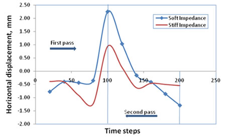
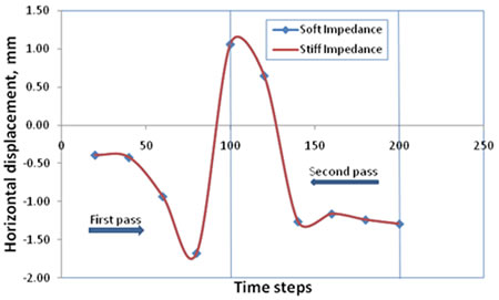
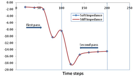
The response plots that have impedance layers around the top fresh mix, old asphalt, and base (as shown in figure 82 and figure 83) are useful in reducing the vertical and horizontal reflections to the point that they are completely eliminated, as indicated in figure 84 and figure 85. Because of this observation, a high enough impedance is sought when use of such layers is warranted, keeping the thickness of layers and the density of the material of the layers fixed.

Figure 82. Chart. Comparison of the dampening effect provided by impedance layers surrounding the structure laterally in the x-direction.

Figure 83. Chart. Comparison of the dampening effect provided by impedance layers surrounding the structure laterally in the y-direction.

Figure 84. Chart. Comparison of the horizontal dampening effect provided by impedance layers surrounding the top layer (pavement and old asphalt) laterally in the x-direction.

Figure 85. Chart. Comparison of the vertical dampening effect provided by impedance layers surrounding the top layer laterally in the x-direction.

Effect of Base Stiffness

FE analyses were performed by assigning properties for the base material in order to study the effect of having a single base layer underneath the pavement. The results indicate that the material response does not seem affected much when the material properties of the single base layer are varied over a wide range with a minimum base stiffness value of 72.5 ksi (500 MPa) and a maximum stiffness value of 290 ksi (2,000 MPa).

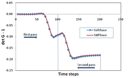
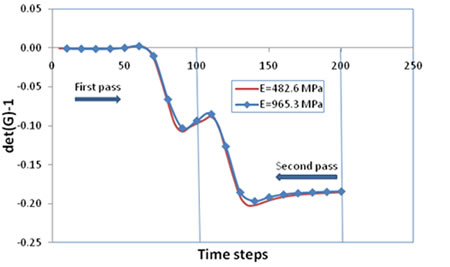
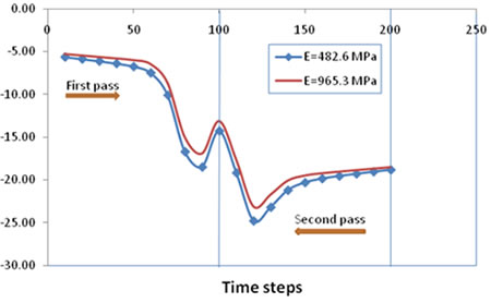
The plots of the volumetric response shown in figure 86 and figure 87 indicate that the material response is not very sensitive to changes in stiffness of the base when the response is viewed in an averaged sense. The volumetric response is examined through the evolution of the volumetric component of the viscous-deformation gradient (see Koneru et al. and Masad et al.).^(48,49) However, the FE model is responsive to a drastic increase in base modulus (as shown in figure 88 through figure 90) due to increasing rigidity in the base structure leading to interference waves (as a result of structural rigidity and not due to any other dynamic characteristic) reflected internally. This is in contrast to what is observed in the field, where mix designs with stiff base materials produce more compaction in the pavement layer because of the compressive reaction acting on the HMA layer from below. As a result, for further FE analysis, a value between the two extremes (i.e., between the minimum base stiffness value of 72.5 ksi (500 MPa) and the maximum stiffness value of 290 ksi (2,000 MPa), for example 145 ksi (1,000 MPa)), is chosen to conduct the parametric and sensitivity analysis presented later.

Figure 86. Chart. Comparison of the volumetric component of the viscous-evolution gradient for soft (72.5 ksi (500 MPa)) versus stiff (290 ksi (2,000 MPa)) bases.

Figure 87. Chart. Comparison of the volumetric component of the viscous-evolution gradient at two base-stiffness moduli of interest.

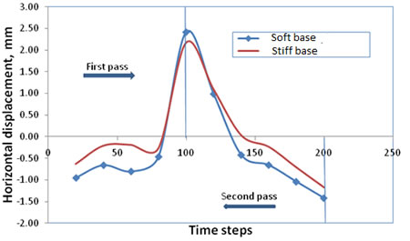
Figure 88. Chart. Comparison of the effect on the x-displacement of a node in the roller path as the base stiffness is varied from 72.5 ksi (500 MPa) (soft base) to 290 ksi (2,000 MPa) (stiff base).

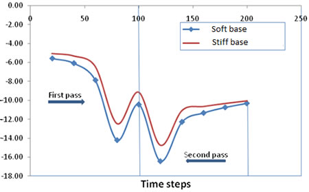
Figure 89. Chart. Comparison of the effect on the y-displacement of a node in the roller path as the base stiffness is varied from 72.5 ksi (500 MPa) (soft base) to 290 ksi (2,000 MPa) (stiff base).

Figure 90. Chart. Comparison of the deflection for two base-stiffness moduli of interest.

Compaction Equipment Characteristics

As a further development to the simulation model, a vibratory-loading algorithm was developed for use in CAPA-3D specifically for the compaction project. The vibratory loads take into account the effect of the displacement amplitude and frequency specifications of the machine used for rolling in a field project by calculating the equivalent load to be used to achieve the same level of compaction. Analytical expressions for calculating the contact forces for cylinder indentation into an elastic pavement material are adapted from Johnson.⁽⁵⁷⁾ Thereafter, the equivalent loads are calculated for different amplitudes of indentation as necessary. Then, the force necessary for the vibrations is calculated using these analytical expressions at an instant of time, and the pressure is redistributed over the contact area.

To summarize, the algorithm has the following features:

• The loading area is the same as the one determined from the static indentation.
• The amplitude of the half-sine, vibratory load is determined based on vibratory-system specifications.
• The time taken for each load cycle is adjusted to match the loading frequency.

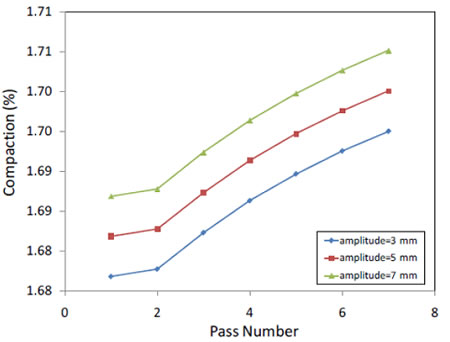
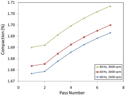
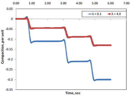
Simulations were set up on a mesh representative of a 12-ft (3.66-m)-wide pavement lane with a roller weight of 27,000 lb (12.258 kg), a diameter of 51 inches (1,295.4 mm), and a width of 7 ft (2.135 m). The results of the simulations (shown in figure 91 through figure 94) show that the material responds according to the mechanics of the loading algorithm implemented. The results are presented at a point in the interior of the material along the width (approximately 5 ft (1.525 m) from the edge). In the results that follow, the term compaction is used as a measure to represent the viscous evolution, det(G)-1 (see Masad et al. for clarification of the term).⁽⁴⁹⁾ The effect of a cyclic load vibrating at a certain angular frequency on the deformation induced on the material model of choice, with a certain relaxation time λ associated with it, is also presented (see figure 94).

The following observations can be made regarding the response of the material:

• An increase in the amplitude of the vibratory load leads to an increase in the amount of compaction achieved (see figure 91).
• The increase in compaction as a result of the increase in amplitude is due to the roller indenting deeper into the material, thereby increasing the pressure on the surface.
• As shown in figure 92 and figure 94, increasing the frequency of the vibration or decreasing the material's viscous nature results in an increase in the percent of compaction of the material, as is observed in the field.
• The response of the material to small steps of increase in load (keeping the roller area of contact constant) results in a uniform increase in compaction level, as indicated in figure 93.

Figure 91. Chart. Compaction over a sequence of passes as the amplitude of vibration increases.

Figure 92. Chart. Compaction over a sequence of passes at different frequencies.

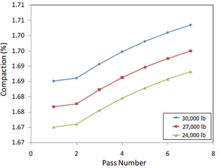
Figure 93. Chart. Material response to change in dead load carried by each roller.

Figure 94. Chart. Field compaction response at a constant frequency over multiple passes on a point.