U.S. Department of Transportation
Federal Highway Administration
1200 New Jersey Avenue, SE
Washington, DC 20590
202-366-4000
Federal Highway Administration Research and Technology
Coordinating, Developing, and Delivering Highway Transportation Innovations
| REPORT |
| This report is an archived publication and may contain dated technical, contact, and link information |
|
| Publication Number: FHWA-HRT-14-061 Date: August 2014 |
Publication Number: FHWA-HRT-14-061 Date: August 2014 |
During field trials for tracking HMA placement described in chapter 3, a small number of the RFID tags rose to the surface of the compacted pavement. This raised the question of whether this would compromise the durability of the pavement by increasing water infiltration or decreasing density locally.
The in-place permeability and density in the local area surrounding surfaced RFID tags were measured to answer this question. The assumption in this evaluation is that if the permeability and density of the pavement around the surfaced tags are similar to that in other areas, it can be assumed that the surfaced tags will not compromise the integrity of the pavement. All of the density and permeability tests were conducted in the UMD Parking Lot EE, where multiple tags surfaced in the 2-inch (50-mm)-thick lift of 0.5-inch (12.5-mm) surface mix (see figure 42).

Original image: ©2015 Google®; map annotations provided by University of Maryland
Figure 42. Photo. Location of permeability and density tests at parking Lot EE at UMD.(7)
In-place density measurements were obtained using the Troxler® Model 3440 nuclear density gauge shown in figure 43. Dr. Nelson Gibson and Mr. Dennis Sixbey of the Federal Highway Administration (FHWA) Turner-Fairbank Highway Research Center (TFHRC) provided the nuclear density gauge and performed the readings at the UMD campus. Mr. Sixbey is a certified nuclear gauge technician as well as the Radiation Safety Officer at the TFHRC. Testing was conducted on July 29, 2009, under generally clear weather conditions.
All nuclear density measurements were conducted in the backscatter mode. It was not possible to calibrate the nuclear gauge because the mix properties were unknown. As a consequence, the absolute density measurements would not be accurate. However, because the main focus of these tests is the relative density near the surfaced tag relative to the density at some distance away, an accurate absolute density reading is not necessary. Two readings were recorded on top of each tag, and 4 additional readings were recorded at distances of approximately 5 inches (125 mm), 9 inches (225 mm), and 16 inches (400 mm) away from the tag (see pattern in figure 44) for a total of 98 readings. Another eight readings were taken at random locations remote from any of the tags. All density measurements were based on 1-min readings. Care was taken to ensure that no vehicles, people, or other potential sources of interference were near the nuclear gauge during the readings. Some of the readings may have suffered some indeterminable loss of accuracy when the roughness of the asphalt surface made it difficult to completely stabilize the device.
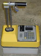
Figure 43. Photo. Troxler® Model 3440 nuclear density gauge.
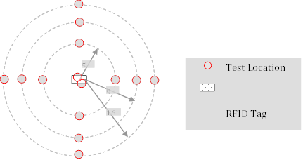
Figure 44. Diagram. Location of tests relative to tag.
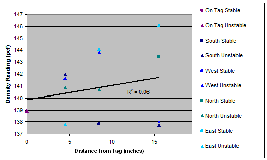
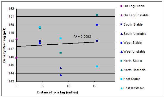
Figure 45 through figure 51 summarize the full set of density readings taken on top of and around each tag. These graphs also indicate which readings might be compromised because of irregularities in the pavement surface.
A linear regression analysis of density versus distance from the surfaced tag was performed for each set of test results. The results are shown as the trend lines in figure 45 through figure 51. The regression line was fit to the entire density data at each distance. However, the slopes of density trends versus distance are the key indicator of interest. The slopes ranged from a minimum of 0.03 for Tag 6 (i.e., essentially no variation of density with distance) to a maximum of 0.18 for tag 3 (i.e., modest variation of density with distance).
There are two reasons to suspect that the measurements directly on top of the tags (i.e., radial distance r equal to 0) may be biased: 1) the tags themselves have lower density than the HMA, so even if the HMA were completely uniform surrounding the tag, the measurements directly on the tag would indicate a lower density for the zone; and 2) the surface irregularities directly surrounding the tag made it more difficult to place the nuclear gauge in a stable configuration directly on top of the tags than in locations away from the tags. To investigate this potential bias, the regression analyses were rerun with the points at r = 0 removed. The slopes for the trend lines with the r = 0 data retained and with the r = 0 data removed are compared in table 9. It is clear that removing the data at r=0 significantly reduces the slope of the density versus distance trend, with some tags now even showing a decrease in density with increasing distance (i.e., tags 5 and 7). The average slope of the trend lines across all tags drops from 0.09 when the r = 0 data are retained to 0.03 when the r = 0 data are removed. In either case, these small slope values suggest very little impact of the tags on in-place density.
As a further check, t- and F-tests were conducted to determine whether there were any statistically significant differences in density at different distances from the tags. These tests compare the means (t-test) and variances (F-test) of two groups of data.
Data for all tags were combined for the purposes of performing the t- and F-tests. To compensate for normal spatial variability of in-place density, the measured density at each location for a given tag was normalized by the average of all density readings for that tag. Any remaining spatial variability after this normalization can then be attributed to distance from the tag. The t- and F-tests were conducted in pairs of datasets: r = 0 (i.e., on top of the tag) and r = 5 inches (125 mm); r = 0 and r = 9 inches (225 mm); r = 0 and r = 16 inches (400 mm); and r = 16 inches (400 mm) and random far-field readings. The results of the t- and F-tests are shown in table 10. The tcrit and Fcrit values in the table are for a significance level α=0.01. In all but one case, both the t- and F-test statistics are smaller than the critical values, indicating that the differences in the means and variances respectively of the two datasets in each pair are not statistically significant. The only exception is the 0 versus 125 mm (5 inches) pair, where the F-test is satisfied but the t value slightly exceeds tcrit. The overall conclusion is that there is very little statistical difference between the density measurements at the various locations from the tag.
pcf = pounds per cubic ft
1 inch = 25.4 mm
Figure 45. Graph. Density as a function of radial distance for tag 1 (slope=0.12).
pcf = pounds per cubic ft
1 inch = 25.4 mm
Figure 46. Graph. Density as a function of radial distance for tag 2 (slope=0.04).
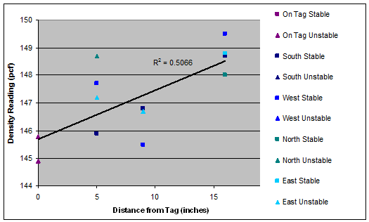
pcf = pounds per cubic ft
1 inch = 25.4 mm
Figure 47. Graph. Density as a function of radial distance for tag 3 (slope=0.18).
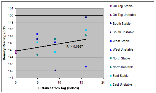
pcf = pounds per cubic ft
1 inch = 25.4 mm
Figure 48. Graph. Density as a function of radial distance for tag 4 (slope=0.11).
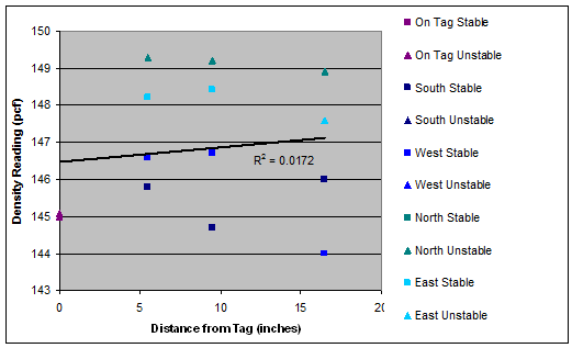
pcf = pounds per cubic ft
1 inch = 25.4 mm
Figure 49. Graph. Density as a function of radial distance for tag 5 (slope=0.04).
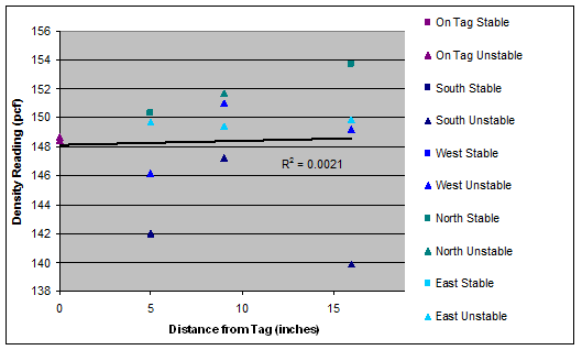
pcf = pounds per cubic ft
1 inch = 25.4 mm
Figure 50. Graph. Density as a function of radial distance for tag 6 (slope=0.03).
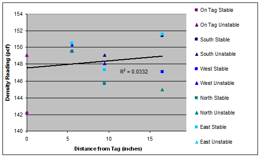
pcf = pounds per cubic ft
1 inch = 25.4 mm
Figure 51. Graph. Density as a function of radial distance for tag 7 (slope=0.08).
Table 9 . Slopes of in-place density versus distance trend lines with and without data at r = 0.
Tag |
Slope |
|
|---|---|---|
With r = 0 Data Points |
Without r = 0 Data Points |
|
1 |
0.12 |
0.05 |
2 |
0.04 |
0.02 |
3 |
0.18 |
0.15 |
4 |
0.11 |
0.10 |
5 |
0.04 |
-0.08 |
6 |
0.03 |
0.06 |
7 |
0.08 |
-0.08 |
Average |
0.09 |
0.03 |
Table 10 . The t- and F-test results for in-place density tests.
Combination |
t |
tcrit |
F |
Fcrit |
|---|---|---|---|---|
0 versus 5 inches |
2.833 |
2.704 |
1.265 |
4.06 |
0 versus 9 inches |
1.741 |
2.704 |
1.538 |
4.06 |
0 versus 16 inches |
2.173 |
2.704 |
3.417 |
4.06 |
16 inches versus far field |
0.465 |
2.727 |
1.049 |
3.86 |
The linear regression analyses of density versus distance at each tag produced very small slope and R2 values in nearly all cases. These both imply little or no relationship between density and distance from the RFID tag. In other words, there do not appear to be any localized variations in in-place density caused by the RFID tags.
The t-tests of the pooled in-place density measurements for all distance combinations except the 0 versus 5 inches (125 mm) case found that any differences in the means were not statistically significant. Even for the 0 versus 5 inches (125 mm) case, the t-statistic exceeded the tcrit value at the 0.01 significance level by only a very small margin. The F values were smaller than Fcrit for all distance combinations, indicating that any differences in variance are not statistically significant. As with the linear regression results, the t- and F-test results suggest that there are no localized variations in in-place density caused by the RFID tags.
In-place permeability tests were conducted on each of the seven surfaced tags using an National Center for Asphalt Technology (NCAT) (Auburn University) field permeameter. The device is centered over the tag and measures the permeability over a diameter of approximately 5.75 inches (145 mm). Seven additional tests were conducted at random locations in the parking lot far from any tags.
The procedure used to conduct the in-situ permeability tests followed the test protocol developed by NCAT.(8) As shown in figure 52, the permeameter consists of four tiers of different diameter cylinders separated in two sections. The sealant used for these tests was plumber's putty. A small 1 ft (0.3 m) square area was identified and brushed clear of debris. A thin layer of the moldable sealant was applied to the rubber gasket on the base plate of the permeameter. Next, a uniform 0.5-inch (12.5-mm)-thick layer of moldable sealant is applied approximately 3 inches (76.2 mm) around the outside diameter on the base plate. Some sealant was reused in other tests after slicing off the top part contaminated by debris. The permeameter is carefully placed on the asphalt test area so that the rubber gasket surrounds the outside diameter of the base plate. Uniform foot pressure is then applied around the perimeter of the base to create a watertight seal with the asphalt.
Many tests were redone because of concern that water observed outside the test area was a leak in the sealant rather than lateral drainage through the HMA. It was sometimes difficult to create a watertight seal because the pavement was uneven. In an effort to improve the seal, four 5-lbf (22.25 N) weights were distributed on the base plate to compensate for the head pressure from the water column. Extra weight was exerted by placing four bricks on the base plate as shown in figure 52.
A thin layer of sealant was used to connect the two sections of the permeameter. The filling tube assembly was inserted all the way to the bottom, and water was added at a steady rate while minimizing bubbles. Water was added until it filled a tier that made it possible for accurate observation of head drop. The time required for the water to drop a given distance in the selected tier was recorded.
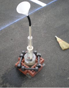
Figure 52. Photo. In-place permeability test setup.
Using the measured time and distance for the water drop, the coefficient of permeability was calculated using the falling head permeability equation shown in figure 53:
![]()
Figure 53. Equation. Permeability determination from falling head permeability test.
where:
k = coefficient of permeability.
a = inside area of standpipe (depends on tier used for testing).
L = thickness of asphalt mat.
A = area of permeameter base through which water can flow into the pavement.
h1 = initial head.
h2 = final head.
t = elapsed time between h1 and h2.
Figure 54 summarizes the results of the 14 permeability tests, which consisted of 7 tests on top of the surfaced RFID tags and 7 random readings far from the tags. Only the reading on top of tag 1 showed a more permeable surface compared with all the other readings. This could be caused by segregation because larger size aggregates were observed on the surface at this location only. Excluding this tag, the readings on top of the RFID tags ranged from 4.92x10⁻⁵ to 41.6x10⁻⁵ inches/s (12.5x10⁻⁵ to 105.6x10⁻⁵ cm/s), which is very similar to the random far-field readings, which ranged from 4.76x10⁻⁵ to 36.8x10⁻⁵ inches/s (12.1x10⁻⁵ to 93.4x10⁻⁵ cm/s). Statistical t- and F-tests were performed to see whether there was any significant difference between the means and standard deviations of these two sets of data. The t-test gave a value of t=0.00813 with tcrit=3.055 at a significance level α=0.01. The F-test gave a value of F=6.87 and Fcrit=8.89. In both cases, the test statistics were less than the critical values, implying no statistically significant differences in the means and variances for the in-place permeability values on top of the RFID tags versus values at random far-field locations.
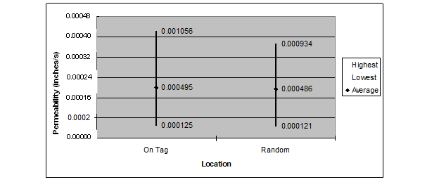
1 inch/s = 25.4 mm/s
Figure 54. Chart. Coefficient of permeability on top of the tags and at random locations.
Based on the very similar ranges in measured permeabilities and the results from the t- and F-tests, it is concluded that there is no detrimental effect of the surfaced RFID tags on in-place permeability for the HMA.
The test results show that there are no practical or statistical impacts on in-place density or permeability from the surfaced RFID tags. Consequently, the tags should not be causes of local damage due to reduced stiffness/strength (correlated with density) or water inflows (related to permeability). Other than aesthetic concerns, the surfaced RFID tags do not appear to have a detrimental effect on asphalt pavements.
There is the possibility for long-term deterioration around the tags due to degradation of the bonds between the asphalt binder and the CPVC pipe encapsulation. However, qualitative observations of the surfaced tags in Lot EE at the time of this writing show no evidence of deterioration over the intervening 6 years.