Radio Frequency Identification Applications in Pavements

CHAPTER 8: GUIDANCE ON DATA INTEGRATION

INTRODUCTION

To ensure-and ideally to improve-the performance of asphalt pavements, it is vital that the influence of material properties on performance be clearly understood. Correlations between as-constructed properties of asphalt concrete in construction databases and field performance of pavements in PMSs can quantify the link between material quality and performance.

Unfortunately, the dissimilar ways in which these two sets of data are recorded with respect to location along the pavement alignment makes it difficult to establish these correlations. As depicted in figure 165, HMA concrete is produced at a production facility and then trucked to the highway construction site for offloading into the asphalt paver. HMA producers sample their production periodically from departing trucks and perform various QC tests to ensure that the mixture properties (gradation, volumetrics) remain within acceptable limits. As part of a QA program, agencies typically take additional samples for acceptance testing to corroborate the producer's QC test results and to establish pay factors. QC and acceptance samples are typically taken at specified tonnage intervals from delivery trucks as they leave the asphalt plant. For example, in Maryland, a minimum of one QC sample (volume sufficient for the full suite of tests) is typically taken for each 1,000-T (909-t) sublot of production. This corresponds roughly to one truck out of every 50 leaving the plant production or approximately 1.25 lane-mi (2 lane-km) of paving for a 2-inch (50-mm) overlay. Test results from this sample are assumed to be representative of the entire 1,000-T (909-t) sublot. One acceptance sample is also taken for each day's production (on the order of 4,000 T (3,636 t) or more). Additional in-place material sampling (cores for field density determination) is also typically performed on the compacted mat. All of these QA material property data can then be stored in the agency's materials management system (MMS) by lot and sublot.

PMS data, on the other hand, are collected at regular intervals during the pavement life after construction and referenced to a specific location in the roadway. For example, in Maryland, an automated distress measurement vehicle (figure 165) collects roughness, rutting, and visual distress data for the entire State highway network on a 2-year cycle. These pavement management data are automatically referenced to the milepoint (or, alternatively, geospatial) location along the roadway.

It is often desirable to compare the PMS distress data during the service life of the pavement with the material property data collected during construction-e.g., for forensic investigations into premature rutting, cracking, or other failures along a particular section of roadway. Unfortunately, at present there is no good practical way to determine precisely where in the roadway the sampled and tested lot/sublot of material was deposited. In many instances, the milepoint range for the entire 1,000 T (909 t) of production represented by the sampled truckload is not even recorded during construction. Unless the HMA QA data can also be tied to a spatial location along the pavement, it cannot be correlated with PMS data on anything better than a crude project-by-project basis.

These problems caused by mismatched referencing of pavement data were highlighted during a pilot implementation of the HMAView software by the MSHA. HMAView is a Web-based application for integrating construction, materials, pavement management, and other pavement data.⁽²⁷⁾ For the pilot project implementation, the spatial location of the QA material property data measured during the original construction had to be laboriously and crudely estimated by hand.

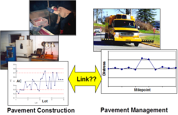
Figure 165. Illustration. Referencing problem in linking pavement construction and pavement management data.

As described in chapters 2 through 4 of this report, inexpensive expendable electronic sensors based on passive RFID technology can be used to identify or tag truckloads of hot mix asphalt as they leave the production plant. These sensors pass through the paver and are compacted into the finished mat. After construction, a vehicle-mounted or handheld scanner is used to electronically "read" the identity tags and cross reference them with latitude and longitude coordinates using GPS technology. These geospatially referenced MMS data can then be directly linked to as-constructed in-place test results and thus to future pavement performance data recorded in the agency's PMS, enabling robust statistical analyses of the correlations between material properties and observed performance.

The application of RFID technology for tracking HMA placement was the genesis for this entire research project. It is also the application that is most suited to near-term commercial implementation. Its major benefit is that it provides a simple and straightforward means for integrating an agency's QA materials property data with its pavement performance measurements. However, several steps are needed to enable this data integration. Given the wide range of materials and pavement management systems in use among the States, the implementation of these steps will be different for each agency. The general guidelines provided in this chapter for the data integration steps can be adapted to each agency's specific database structures, policies, procedures, and information technology infrastructure.

GUIDELINES FOR INTEGRATING MMS AND PMS DATABASES

A wide variety of MMSs and PMSs have been implemented by highway agencies nationwide. In some cases, these systems may have been developed in-house, either by agency personnel or by consultants, and subsequently modified and extended over time. This makes it difficult to develop a "one size fits all" set of guidelines for integrating these two sets of data. Therefore, the approach adopted here is to outline the general set of issues that must be addressed when integrating these two data sources and to illustrate them, where possible, using application examples from AASHTOWare™'s SiteManager™ product, Fugro's Roadware/Vision software, the MSHA MarylandWare software, and other sources from the literature and, where appropriate, database examples using Microsoft® Access.^(28,29) (The Microsoft® Access 2007 version is used.) The SiteManager™ and Roadware/Vision software, in particular, are used by a significant number of State transportation departments for materials management and pavement management/data display, respectively.

The basic components required for implementing an RFID-based HMA materials tracking system and for integrating MMS and PMS databases are as follows:

1. Linkage of RFID identifiers to material samples collected at the plant or in the field.
   
   
2. Linkage of GPS latitude and longitude coordinates to RFID identifier and thus to the material sample.
   
   
3. (Optional) Conversion of latitude/longitude to PMS location reference system (e.g., milepoints).
   
   
4. Extraction of MMS and PMS data by roadway location.
   
   
5. Display of extracted data for data analysis and other purposes.
   
   

Each of these components is discussed in more detail in the following subsections. The focus here is on QA material samples taken from RFID-tagged trucks as they leave the HMA production plant and the material property tests that are obtained from these samples. QA samples taken directly from the roadway are not considered here because the spatial location of these samples is known directly although they may not be recorded to allow linkage with the PMS. The terms used in these discussions are defined as follows:

• Tag: An RFID tag placed in a sampled transport truck as it leaves the HMA production plant. For redundancy, there will generally be multiple tags in a single transport truck.
  
  
• Tag ID: The digital identification label that is electronically coded into each RFID tag.
  
  
• Material sample (or sample): The material sampled from a single truck as it leaves the HMA production plant. It is assumed here for simplicity that there is one sample per truck, but the logic could be easily generalized to multiple samples per truck.
  
  
• Test: A QA material property test obtained for a material sample. There will in general be multiple QA material property tests (e.g., asphalt content, maximum specific gravity, etc.) associated with a material sample.
  
  
• Join: The relational database operation that combines information from multiple database tables based upon common data elements shared by the tables (e.g., ID fields).
  
  

Linkage of RFID Identifier to Material Samples

For redundancy, multiple RFID tags are deposited in each sampled truck as it leaves the plant because some of the tags may fail or be unreadable after being compacted into the roadway. In addition, multiple test specimens and test types may be associated with each sample in the MMS. The following two types of relationships must therefore be addressed:

• The many-to-one relationship between RFID tags and material samples.
  
  
• The one-to-many relationship between a material sample and the various test specimens that are prepared from the material sample.
  
  

Dealing with the second issue first, this classic one-to-many data relationship is incorporated directly into most MMSs, including the SiteManager™ Laboratory Inventory Management System (LIMS) module. In SiteManager™ LIMS, a sample ID is established first and then multiple test types are associated with it, as shown in figure 166. This can also be accomplished using a standard relational database join operation as illustrated schematically in figure 167 through Figure 169. The query, given both in terms of the Microsoft® Access 2007 query designer and its Structured Query Language equivalent, extracts the three material property values (two asphalt contents and one voids in the mineral aggregate measurement) from tests performed on material from sample 54321. Note that the query in figure 168 can be implemented in other and arguably more efficient ways; the particular query structure in figure 168 is designed to highlight the one-to-many relationship between material samples and material property tests.

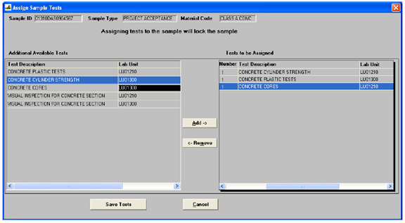
Figure 166. Screen Capture. Assign Sample Tests screen from SiteManager™ LIMS.

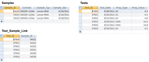
Figure 167. Screen Capture. Schematic for associating a single sample (Sample_ID=54321) with multiple test specimens/material properties (Microsoft® Access 2007): Samples, Tests, and Test_Sample_Link tables.

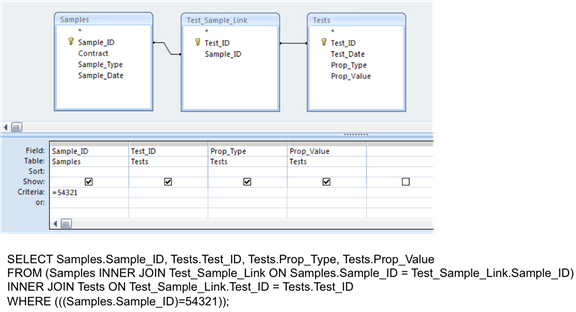
Figure 168. Screen Capture. Schematic for associating a single sample (Sample_ID=54321) with multiple test specimens/material properties (Microsoft® Access 2007): Query.

Figure 169. Screen Capture. Schematic for associating a single sample (Sample_ID=54321) with multiple test specimens/material properties (Microsoft® Access 2007): Query results.

The second issue of associating potentially multiple RFID tags IDs to a single material sample can be handled in either of two ways:

1. Because the multiple RFID tags are intended to be redundant, only one of the readable tags in the set can be selected as representing the entire set. The linkage between RFID tags and material samples then simplifies to a one-to-one relationship. The tag ID can then be simply included as another data element in the material samples table.
   
   
2. If it is desirable to maintain the redundancy between tags and samples, a linking table and associated join operations can be established between RFID tags and material samples and thus between tags and test specimens, as illustrated schematically in figure 170 through figure 172. The Tag_Sample_Link table captures the many-to-one relationship between tag IDs and samples. The query passes this additional information along, generating a table of tag IDs and the material property values measured for all tests from the sample associated with the tag IDs.
   
   

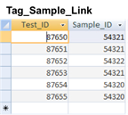
Figure 170. Screen Capture. Schematic for associating multiple RFID tags with a single material sample (Sample_ID=54321) having multiple test specimens/material properties (Microsoft® Access 2007): Tag_Sample_Link table (see figure 169 for other tables in query).

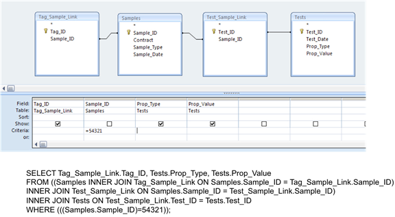
Figure 171. Screen Capture. Schematic for associating multiple RFID tags with a single material sample (Sample_ID=54321) having multiple test specimens/material properties (Microsoft® Access 2007): Query.

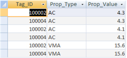
Figure 172. Screen Capture. Schematic for associating multiple RFID tags with a single material sample (Sample_ID=54321) having multiple test specimens/material properties (Microsoft® Access 2007): Query results.

Linkage of GPS Coordinates to RFID Identifier/Material Sample

By definition, there is a one-to-one relationship between GPS coordinates and an RFID tag ID-i.e., the RFID tag can only be in one spatial location. The GPS coordinates can be entered directly into the Tags table after the tag has been interrogated by the vehicle-mounted reader and antenna system after construction.

The linkage of GPS coordinates to material samples is a bit more difficult. As described in the preceding section, there may be one or more RFID tag IDs associated with a single material sample. Consequently, there may be one or more sets of GPS coordinates associated with each single material sample. This issue can be addressed via one of three possible approaches:

1. Single RFID tag/single set of GPS coordinates: Most MMSs permit entry of one-to-one location links for material samples. The current version of the SiteManager™ LIMS and the MarylandWare QC/QA module permit direct entry of latitude and longitude for a sample; an example from the MarylandWare QC/QA module is shown in figure 173. The single set of latitude and longitude coordinates can be simply entered manually into the material sample screens. Alternatively, software utilities can be developed locally to automate entry of the latitude and longitude coordinates from the tags table.
   
   
2. Multiple RFID tags/sets of GPS coordinates: This can be handled in any of three ways:
   
   
   1. Because the multiple RFID tags are intended to be redundant, only one of the readable tags in the set can be selected as representing the entire set. The linkage between the GPS coordinates for the selected RFID tag and material samples then simplifies to a one-to-one relationship. Entry and storage of the GPS coordinates in this case is similar to that in the preceding item 1.
      
      
   2. Average or "best estimate" latitude and longitude values can be determined for the multiple redundant RFID tags associated with one sample. The linkage between the best-estimate GPS coordinates and material samples then simplifies to a one-to-one relationship. Entry and storage of the GPS coordinates in this case is similar to that in the preceding item 1.
      
      
   3. If it is desirable to maintain the redundancy between tags/sets of GPS coordinates and samples, a linking table and associated join operations can be established between the RFID tags/GPS coordinates and material samples and thus between tags/GPS coordinates and test specimens, as illustrated schematically in figure 174 through figure 176. The new Tags table contains the tag ID and associated latitude and longitude. The Tag_Sample_Link table captures the many-to-one relationship between tag IDs/GPS coordinates and samples. The query then uses this information to generate an output table listing for each tag the multiple material property test results determined from the material sample associated with that tag. As before, the query in figure 175 can be implemented in other and arguably more efficient ways; the particular query structure in figure 175 is designed to highlight the many-to-one relationship between RFID tags and material samples and the one-to-many relationship between material samples and material property tests.
      
      
   
   
   

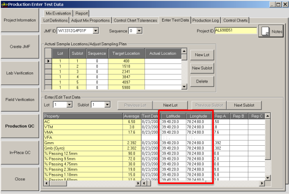
Figure 173. Screen Capture. MarylandWare example of direct entry of latitude and longitude location for a material sample (boxed area of screen).

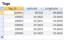
Figure 174. Screen Capture. Schematic for associating multiple sets of GPS coordinates with a single material sample (Sample_ID=54321) having multiple test specimens: Tags table, augmented with GPS coordinates (see figure 167 and figure 170 for other tables in query).

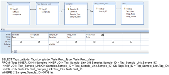
Figure 175. Screen Capture. Schematic for associating multiple sets of GPS coordinates with a single material sample (Sample_ID=54321) having multiple test specimens: Query.

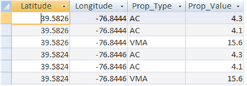
Figure 176. Screen Capture. Schematic for associating multiple sets of GPS coordinates with a single material sample (Sample_ID=54321) having multiple test specimens: Query results.

Conversion of Latitude/Longitude to Roadway Location

The spatial referencing of the tags, and therefore of the associated material samples and material property test results in the MMS, are in terms of two-dimensional latitude and longitude. However, PMS data are most commonly spatially referenced in terms of linear milepoints along a route. Therefore, it is necessary to convert latitude and longitude to route and milepoint if the MMS data are to be combined with the PMS data. This is typically done by pairing GPS coordinates with milepoint locations at key points along the route and then interpolating. More information can be found in Schwartz and Bentahar and in O'Neill and Harper.^(30,31)

Fortunately, most PMS software (including Roadware/Vision) already incorporates such coordinate conversion routines. In part, this is because some important PMS data elements-e.g., falling weight deflectometer test data as collected using Dynatest® and other common commercial systems-are spatially located automatically in terms of GPS coordinates. The material property data measured during construction can thus be exported from the MMS and imported into the PMS, and the PMS conversion routines can translate the GPS coordinates to milepoints. All MMSs and PMSs incorporate some type of data export/import routines, although there may be formatting incompatibilities that would need to be resolved on an agency-by-agency basis.

Combining MMS and PMS Data by Location

Once the GPS coordinates for the MMS data have been converted to milepoints within the PMS, they can be extracted and combined with any desired PMS data elements. This would typically be done using the query facilities built into the PMS. Figure 177 through figure 179 illustrate schematically how to extract both MMS and PMS data along a particular section of roadway. New Route_No and Milepoint data elements have been added to the Tags table; the latitude and longitude coordinates and the PMS spatial reference conversion routines are used to generate the values for populating these data elements. The query in figure 177 through figure 179 is similar to that in figure 174 through figure 176, with the only difference being the reporting of route number and milepoint instead of latitude and longitude for each material property test value.

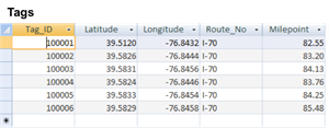
Figure 177. Screen Capture. Schematic for extracting MMS data along a portion of roadway (I-70 between milepoints 83 and 84): Tags table, augmented with milepoint data elements (see figure 167 and figure 170 for other tables in query).

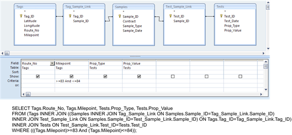
Figure 178. Screen Capture. Schematic for extracting MMS data along a portion of roadway (I-70 between milepoints 83 and 84): Query.

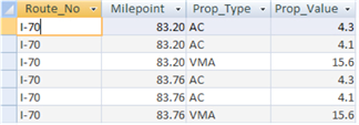
Figure 179. Screen Capture. Schematic for extracting MMS data along a portion of roadway (I-70 between milepoints 83 and 84): Query results.

Figure 180 through figure 182 show a simple example query for extracting International Roughness Index (IRI) values from a PMS database. The output from the query lists the measured IRI values and associated milepoint along the specified section of roadway.

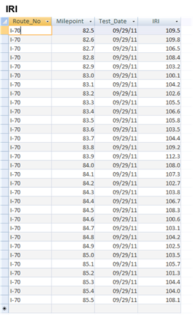
Figure 180. Screen Capture. Schematic for extracting PMS data along a portion of roadway (I-70 between milepoints 83 and 84): IRI table.

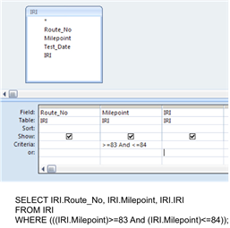
Figure 181. Screen Capture. Schematic for extracting PMS data along a portion of roadway (I-70 between milepoints 83 and 84): Query.

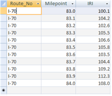
Figure 182. Screen Capture. Schematic for extracting PMS data along a portion of roadway (I-70 between milepoints 83 and 84): Query results.

Display of Extracted Data

Once the MMS and PMS data have been extracted as described in the preceding section, they can be displayed together, typically using the built-in data display routines in the PMS. Figure 183 shows a Roadware iVision display of multiple datasets versus milepoint location along the roadway. One of the data series in the lower left chart or the data series in the lower right chart in the figure could be replaced by one of the MMS data elements, e.g., asphalt content as measured during construction.

The exported MMS and PMS data can also be exported for subsequent external analyses. Most PMSs have the capability of exporting query results, often through some type of "report generator" feature. The available formats for the output data will vary from system to system.

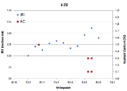
Figure 184 is an example of using Microsoft® Excel for displaying the extracted PMS and MMS data. The PMS data elements (IRI) and MMS data elements (asphalt content) are displayed as separate series (and with separate y-axes). The data in figure 184 are consistent with those in the earlier schematic examples in figure 177 through figure 182. An examination of figure 184 suggests that the localized higher roughness around milepoint 83.9 may be associated with a low and/or variable asphalt content. These types of insights, many of which will be far more powerful than in these simple examples, are the key benefits of integrating MMS and PMS data.

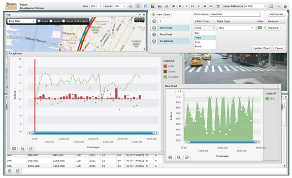
Figure 183. Screen Capture. Roadware iVision charts screenshot.⁽²⁹⁾

1 inch/mi = 0.041 m/km
1 mi = 1.61 km
Figure 184. Graph. Roughness (IRI) from PMS and asphalt content from MMS along a specified section of roadway (I-70 between milepoints 83 and 84).

DATA INTEGRATION SUMMARY

Maximum use of material property data collected during construction and pavement management data collected during service life is possible only when both sets of data can be related to a common spatial referencing system. Using RFID tags to track loads of sampled and tested material enables geospatial identification of the location of the delivered material in the pavement. These material properties can then be linked with the corresponding spatially located pavement performance data from the PMS.

Because of the wide variety of MMS and PMS used by agencies, it is possible only to outline the general steps to link these two datasets via geospatial coordinates. This chapter provides examples of the following necessary operations:

• Linkage of one or more RFID identifiers to material samples.
  
  
• Linkage of GPS coordinates to RFID identifier/material sample.
  
  
• Conversion of latitude/longitude to roadway location.
  
  
• Combining of MMS and PMS data by location.
  
  
• Display of extracted data.
  
  

The details of implementing these operations will depend on the particular MMS and PMS used by an agency.