Radio Frequency Identification Applications in Pavements

CHAPTER 6: PAVEMENT TEMPERATURE MEASUREMENT USING SAW RFID

INTRODUCTION

There have been efforts since the late 1960s to model HMA temperatures as a function of time as an aid to optimizing compaction. Compaction is a densification process in which the air voids in an HMA mixture are reduced by the application of mechanical energy, commonly via a vibratory steel-drum roller. It is widely recognized that compaction is a critical factor in flexible pavement performance. Achieving optimal compaction for any particular mix depends primarily on temperature (for a given asphalt viscosity) and compactive effort. Inadequate compaction may result in reduced pavement stiffness, fatigue life, and durability.

Temperature versus time during compaction is especially important when using state-of-the-art intelligent compaction techniques. One of the principal advantages of intelligent compaction is the estimated stiffness of the compacted material as determined from the feedback sensors on the vibrating drum. The stiffness of HMA (and also warm mix asphalt) is extremely dependent on temperature. Analysis of the feedback data from the sensors on the intelligent compactor thus requires knowledge of the temperature distributions with depth and time in the cooling mat. The conventional infrared temperature measurements taken during compaction measure only the temperature at the surface-the coolest location in the mat-and may be biased by the water sprayed on the rollers. A technique for measuring temperature throughout the mat thickness in real time has potential for improving the effectiveness of intelligent compaction for asphalt concrete.

The specific objectives of the investigations reported in this chapter are as follows:

1. Evaluate the feasibility of using SAW-based RFID technology to measure HMA temperatures versus depth and time via wireless sensors.
   
   
2. Demonstrate, both in the laboratory and the field, the survivability and temperature measurement capabilities of the SAW RFID sensors.
   
   
3. Perform analyses of the measured field data to develop asphalt cooling curves (temperature versus time) and compare these results with analytical mat cooling models. The coupling of some limited field measurement data with analytical models leverages the value of the sensor data.
   
   
4. Perform a sensitivity analysis on the input parameters for the traditional mat cooling models and calibrate, via the sensitivity analysis, input parameters that provide reasonable and close agreement with the measured temperatures from the field.
   
   

This work was performed in conjunction with the FHWA Pooled Fund Study on Intelligent Compaction and specifically with an intelligent compaction demonstration project conducted in Maryland.⁽¹³⁾

PREVIOUS WORK

A literature review of all previous work related to the development mat cooling models was performed. Although numerous journal articles and technical reports were reviewed, only the most relevant to the present study are discussed here.

Heat Flow Formulations

Corlew and Dickson pioneered methods for predicting HMA temperatures as a function of time from when the asphalt leaves the paver to the end of compaction.⁽¹⁴⁾ Their mat cooling model is based on the principles of one-dimensional transient heat flow as illustrated in figure 63.

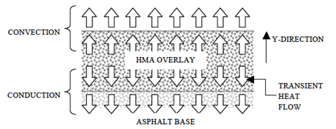
Figure 63. Drawing. Cross section of an HMA overlay indicating directional flow of thermal energy.

Transient heat flow is described by the partial differential equation (PDE) relating temperature T, time t, and depth y shown in figure 64.

Figure 64. Equation. Differential equation for transient heat flow.

The parameter α in figure 64 is the thermal diffusivity-the ability of a material to conduct thermal energy compared with its ability to store thermal energy. The equation in figure 65 defines thermal diffusivity:

Figure 65. Equation. Definition of thermal diffusivity.

where:

k = thermal conductivity of the material.
ρ = material density.
C_p = specific heat capacity.

The units for thermal diffusivity are area per unit of time (e.g., ft²/h).

Although Corlew and Dickson proposed an analytical solution to the equation in figure 64, they found that the interactions of the various modes of thermal energy transfer at the pavement surface were better modeled using numerical techniques.

Figure 66 illustrates the numerical solution scheme for the transient heat flow analysis. The pavement thickness is divided into sublayers (sections divided by isothermal lines) and the PDE in figure 64 is approximated using finite difference equations at the nodes located at the midpoints of each sublayer. As shown in figure 66, the nodes extend from the pavement surface boundary through the overlay and continue for some depth through the asphalt base to the lower boundary. The boundary conditions consist of a constant ambient air temperature (T_Air) above the surface of the overlay (depth location i=n) and a constant base temperature at the bottom of the analysis domain (i=1). The lower boundary is located at a sufficient depth where conduction no longer affects the temperature of the base material over the duration of the transient analysis-i.e., the bottom boundary condition is T_1j = T_Initial for all time steps j.

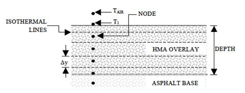
Figure 66. Drawing. Typical incremental elements of HMA overlay used in numerical solution.

Figure 67 expresses the finite difference approximation of the heat balance equation within the mat:

Figure 67. Equation. Finite difference approximation to heat balance equation.

where:

i =2...n-1 = the node number in the interior.
T_ij = temperature (°F) at node i and time j.

The equation in figure 68 solves for T_i,j+1.

Figure 68. Equation. Equation for T_i,j+1.

These one-dimensional conduction equations are used to calculate temperatures within both the HMA overlay and the asphalt base. Corlew and Dickson point out that the thermal diffusivity might be different for the two materials. However, this difference is expected to be small for most asphalt mixtures. Therefore, the thermal diffusivity is assumed uniform for the overlay and base material.

Similarly to conduction, heat loss from the surface i=n due to convection and radiation is based on the energy balance equation shown in figure 69:

Figure 69. Equation. Energy balance equation for convective and radiation heat losses at pavement surface.

where:

N_B = Biot number (described below).
k = thermal conductivity (BTU/ft²-h-°F/ft).
T_Air = ambient air temperature (°F).
α = solar absorptivity.
H_S = solar heat flux (BTU/ft²-h).
ε = emissivity.
σ = Stefan-Boltzman constant-1.713x10^-9 (BTU/ft²-h-°R⁴).

The Biot number is a dimensionless value commonly used in transient heat flow and mass transfer analysis.⁽¹⁵⁾ It is the ratio of heat transfer resistances within and at the surface of a mass undergoing convection. This number indicates whether temperatures within the body will vary significantly in space while the mass heats or cools over time due to thermal energy transfers at its surface. Mathematically, the Biot number is defined as the equation shown in figure 70.⁽¹⁵⁾

Figure 70. Equation. Definition of Biot number.

The convective heat transfer coefficient h in figure 70 relates convective heat flow with temperature difference and surface area via Newton's law of cooling. The effective length s is the ratio between volume and surface area, and k is the thermal conductivity. The final radiation term in figure 69 includes parameters that account for the absorption of radiant solar energy (a H_S) and for the radiant energy emitted by the pavement (ε σ).

Corlew and Dickson developed a computer program to simulate mat cooling based on this finite difference formulation. To validate this model, they performed field experiments in which thermocouples were embedded throughout the depth of an HMA overlay to measure mat cooling versus time. Wind velocity, ambient air temperature, initial base temperature, solar radiation, and overlay thickness were also measured in their experiments. Corlew and Dickson found very close correlations between measured and predicted temperatures.

Overall, Corlew and Dickson's study suggested the following:

1. When using proper environmental conditions, modeling mat cooling is feasible and accurate using finite difference analysis techniques.
   
   
2. The heat flux from the overlay into the underlying base layer is initially greater than the heat flux into the atmosphere. Therefore, the lower region of the overlay expels heat faster than the upper region. However, Jordan and Thomas found that with increasing time, the cooling of the surface becomes dominant.⁽¹⁶⁾
   
   

Wolfe and Colony expanded on Corlew and Dickson's approach and converted the mat cooling models into a format more suitable for the portable handheld computers of the time and for tabular and graphical summary.⁽¹⁷⁾ In an attempt to streamline the conductive heat flow calculations in figure 68, Wolfe and Colony used Saul'yev's method for conduction, a numerical technique based on forward and backward finite differences. Saul'yev's method requires less memory than that needed by Corlew and Dickson's formulation and thus was better suited to the comparatively primitive handheld computers available in the 1970s. Wolfe and Colony also developed an explicit form of convective heat transfer energy balance at the mat surface.

Wolfe and Colony also employed the slightly different finite difference energy balance equation shown in figure 71 for the heat flows at the surface of the mat. All terms were as defined previously.

Figure 71. Equation. Modified version of finite difference energy balance for heat flows at surface of mat.

Figure 71 includes energy losses due to radiation and convection and gains from solar radiation. Figure 71 can then be rearranged as shown in figure 72 to solve for the temperature at the next time step, T_n,j+1.

Figure 72. Equation. Modified equation for T_n,j+1 at mat surface.

Figure 68 and figure 72 are used in this study as the finite difference solution for the transient heat flow in the overlay.

Wolfe and Colony argued that both free and forced convection effects should be included when calculating the convective heat transfer coefficient.^(17,18) Free convection occurs when there is no wind velocity, as opposed to forced convection that includes wind velocity. Wolfe, Heath, and Colony recommended the relationship shown in figure 73 for convection⁽¹⁹⁾:

Figure 73. Equation. Relationship for forced convection.

where V is the wind velocity in mi/h.

Wolfe and Colony state that solar heat flux emitted by the Sun can range up to about 400 BTU (422 kJ) per hour at local solar noon.⁽¹⁷⁾ However, it is dependent on the time of the year, the Sun's declination, and the location (latitude) of the surface being considered. They suggest the the equation in figure 74 for estimating solar heat flux⁽¹⁸⁾:

Figure 74. Equation. Relationship for estimating solar heat flux.

where:

R =incident solar radiation (direct and diffuse).
N = a cloud base factor, which varies from 0.80 to 0.90.
W = percentage cloud cover, which is visually estimated.

The value for incident radiation is obtained from historical data. The authors provide a graph of solar heat flux versus time for typical incident radiation in Ohio between 38°50' and 42°00' latitude (the location of their study).

Alternative methods for determining solar heat flux have been proposed in the literature. Rather than modifying solar radiation for cloud effects and cover, radiation can also be quantified in terms of the effective sky temperature.⁽²⁰⁾

Wolfe, Heath, and Colony performed laboratory and then field tests to demonstrate that their numerical predictions correlated favorably to measured mat cooling curves.⁽¹⁹⁾ The field trials were performed in November 1979 at a project site in Ohio. The field instrumentation at the project site included a radiation pyrometer to measure base surface temperatures, a pyrheliometer to measure solar insolation, an anemometer to measure wind speed, temperature probes, and recording devices. Field temperatures were measured near and at the interface of the newly placed HMA and its base layer. Surface temperatures were also measured but were dismissed because of instrument inaccuracies. The field test found generally close correlations between calculated and measured temperatures.

Wolfe, Heath, and Colony concluded that their predictive equations were adequate for the purpose of making "go/no-go" decisions in the field for placing and compacting HMA under adverse site conditions.⁽¹⁹⁾ Specific findings from the study included the following:

• Based on the simulation results, solar radiation and cloud cover are not major influences on the placement of HMA. In other words, solar radiation should not be considered in making a "go/no-go" decision in the field.
  
  
• The convective heat transfer coefficient is relatively difficult to measure. There are numerous equations and experimental methods to estimate this parameter. However, the study generally confirmed the recommendations in figure 73 for this value.
  
  
• Prior to the actual paving, the surface of the base material is subjected to heat from the paver as it passes. The authors suggested that, depending on the speed of the paver (and if it pauses), the initial interface temperature between the asphalt and base material may not be accurate. Temperatures should be recorded once the paver passes the test area.
  
  

Thermal Property Values

Wolfe and Colony, based on a review of several sources, recommended typical values for other thermophysical material properties of asphaltic mixtures.⁽¹⁷⁾ These are summarized in table 14.

Table 14 . Typical thermal property values.⁽¹⁷⁾

N/A = Not Applicable
1 BTU/ft-h-°F = 1.73 W/m-°K
1 ft²/h = 0.093 m²/h

Luca and Mrawira performed a series of laboratory tests to measure the thermal diffusivity α and thermal conductivity k for Superpave HMA mixtures and compared their measured values with values reported previously in the literature.⁽²¹⁾ Their measured values generally agreed favorably with those in the literature; the values fit within a general range of 1.35x10^-2 to 3.20x10^-2 ft²/h (1.25x10^-3 to 2.98x10^-3 m²/h) for thermal diffusivity and 0.70 to 2.24 BTU/ft-h-°F (1.21 to 3.88 W/m-°K) for thermal conductivity. The authors highlight that these parameters are generally difficult to measure. Table 15 and table 16 summarize Luca and Mrawira's findings.

Table 15 . Typical values for thermal diffusivity.⁽²¹⁾

Table 16 . Typical values for thermal conductivity.⁽²¹⁾

LABORATORY EVALUATION OF SAW RFID TAGS

The differences between surface SAW and conventional RFID were described in chapter 1. A series of laboratory tests were performed to evaluate the suitability of SAW RFID technology for pavement applications. These tests were organized into the following subtopics:

• Development of an encapsulation process using thermally conductive epoxy that will promote the transfer of thermal energy while protecting the tag from physical damage.
  
  
• A read range study to evaluate the signal strength/readability of the SAW RFID tags. The read range study includes testing for tag orientation (including rotation) to the antenna and position/distance from the antenna.
  
  
• A thermal sensitivity study to evaluate the thermal response of the tags when exposed to elevated temperature transients. More specifically, this study evaluates the time required for a tag to heat up and then equilibrate to the temperature of the surrounding material/ environment.
  
  

Tag Encapsulation

Encapsulating the RFID tags with a thin coating of thermally conductive epoxy protects them from paving and compaction stresses while only minimally interfering with heat transfer during mat cooling. The encapsulation medium selected for this study is Durapot 865™ epoxy from Cotronics, Inc. This encapsulant has a thermal conductivity of about 1 BTU/ft-h-°F (1.73 W/m-°K) and is electrically insulating. To put this parameter into perspective: the thermal conductivity of copper is about 230 (400), standard epoxy is about 0.20 (0.35), and asphalt is about 0.433 BTU/ft-h-°F (0.75 W/m-°K). Durapot 865™ is a two-component epoxy (resin and hardener) that cures at room temperature. The following encapsulation procedure was used:

• The epoxy resin component is preheated for about 40 min at 122 °F (50 °C) to reduce its viscosity.
  
  
• The epoxy components are then combined at 100 parts resin to 21 parts hardener and thoroughly mixed.
  
  
• The wooden mold (fabricated in advance) is lined with standard kitchen plastic wrap secured using masking tape.
  
  
• A layer of epoxy is poured at the bottom of the mold prior to tag placement to create a thin protective base layer.
  
  
• The tag is placed in the mold on top of the bottom epoxy layer and pressed downward into the encapsulant. The tag is then covered in the epoxy to completely encase it.
  
  
• The wood mold, with epoxy and tag, is then placed in a vacuum dessicator to remove any air pockets in the epoxy.
  
  
• After removing the air and curing for 24 hours, the tags are removed and sanded for smoothness.
  
  

Figure 75 shows the unencapsulated tags used in this study. As will be described more fully later, the larger tag on the left of figure 75 is the single patch antenna tag (with larger receiving antenna) approximately 45 by 45 mm (1¾ by 1¾ inches) in size. The tag on the right is the monopole antenna tag approximately 8 by 45 mm (1/3 by 1¾ inches) in size. Figure 76 shows the encapsulated tags prior to final sanding. Both unencapsulated and encapsulated tags were evaluated in the read range and thermal sensitivity studies.

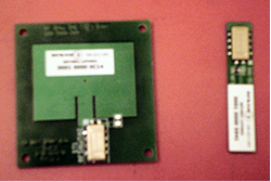
Figure 75. Photo. Unencapsulated RFID tags (left: single patch, right: monopole).

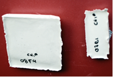
Figure 76. Photo. Encapsulated RFID tags before finish sanding (left: single patch, right: monopole).

Signal Strength and Readability

A series of read range tests were performed to evaluate the signal strength and readability of the SAW RFID tags in both the monopole and single patch antenna configurations. The monopole and single patch tag antennae differ primarily in the shape of their RF field distributions (for transmission) and sensitivities (for reception).

The monopole antenna is formed by replacing half of its dipole antenna with a ground plane normal to the antenna axis. If the ground plane is sufficiently large, the monopole behaves like a dipole with its reflection in the ground plane providing the missing symmetric half. A dipole antenna has a toroidal field strength/sensitivity distribution with omnidirectional field strength/ sensitivity in the midplane and normal to the antenna axis, and with dead zones at the ends of the dipole.

Patch antennae, on the other hand, are designed for a more directional RF radiation/sensitivity. A simple patch antenna consists of a looped antenna one-half wavelength long, separated by a constant thickness over a ground plane. The ground plane is typically only modestly larger than the active patch. The simple patch antennae of this type radiate a linearly polarized wave. The typical radiation pattern for a linearly polarized patch antenna is unidirectional with a beam width angle of about 65 degrees. An infinitely large ground plane would prevent any radiation toward the back of the antenna. But, with the more usual finite ground plane, power loss through the back side of the antenna is about -20 dB compared with the front side.

Two types of reader antennae were supplied with the SAW RFID system-linearly and circularly polarized. Both reader antenna types were evaluated for the following tag configurations: unencapsulated tags in air, encapsulated tags in air, and encapsulated tags in an asphalt specimen.

Unencapsulated Tags in Air

To determine the full read range capacity of the unaltered SAW RFID tags, an "open-floor" read range study was performed. The following diagrams illustrate the read range capacity for the unencapsulated tags in air. Each cell within the diagram represents a 1 ft (0.3 m) interval of lateral offset or distance ahead of the antenna. Note that the antenna is fixed 1 ft (0.3 m) away from the test grid in front of cells L-A and R-A. For example, cell "-2, B" is located 2 ft (0.6 m) to the left and 3 ft (1 m) ahead of the face of the antenna. The numbers in each cell are the number of read responses from the tag at that location during a 20s interval.

A uniform tag orientation was used throughout this study. The tag was affixed to the back of a plastic board, antenna oriented vertically, facing toward the reader antenna (unless otherwise noted). Figure 77 and figure 78 display the results of the read range study performed on a single patch tag using a linearly polarized antenna and circularly polarized antenna, respectively. The green cells indicate strong reliable readings, yellow are more unpredictable, and red are zero or unlikely readings. Figure 79 and figure 80 summarize the corresponding read range results for unencapsulated monopole tags using a linearly and circularly polarized antenna.

Comparing these four figures, it is apparent that the single patch tags have a stronger readability than the monopole tags, both in terms of the number of reads and the width of the readable zone ahead of the antenna. This is because of the larger size and higher sensitivity of their antennae. However, all of the unencapsulated tags (patch and monopole) exhibited read ranges greater than 8 ft (2.4 m) in air.

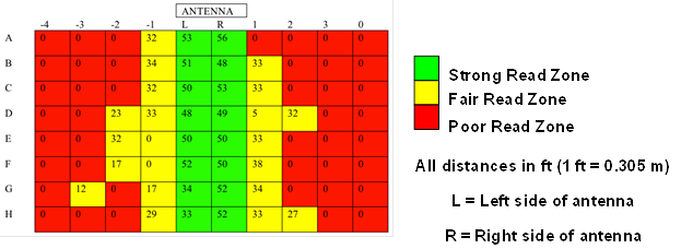
Figure 77. Diagram. Unencapsulated single patch tag, linear polarization.

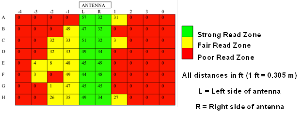
Figure 78. Diagram. Unencapsulated single patch tag, circular polarization.

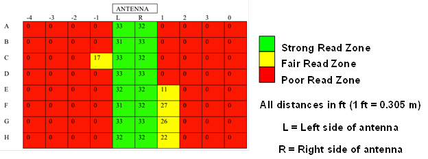
Figure 79. Diagram. Unencapsulated monopole tag, linear polarization.

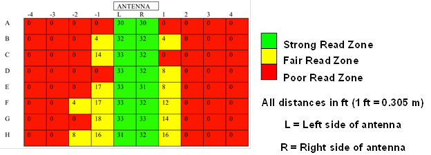
Figure 80. Diagram. Unencapsulated monopole tag, circular polarization.

Encapsulated Tags in Air

Similar read range testing was performed on tags after encapsulation in thermally conductive epoxy. Figure 81 and figure 82 summarize the measured read ranges for the encapsulated single patch tag using linear and circular reader antenna polarization, respectively. Figure 83 and figure 84 summarize similar results for the encapsulated monopole tag.

Based on the results in these figures, it is again apparent that the single patch tags have better readability than the monopole tags. In addition, the polarization of the reader antenna influences read performance. A linearly polarized antenna has more directionality than the circularly polarized antenna. This means that, all else being equal, the linearly polarized antenna will have better read performance for some orientations of the tag (relative to the plane of the antenna polarization) and worse read performance for others, compared with the circularly polarized antenna. In general, the circularly polarized antenna will have slightly lower read performance but with much less sensitivity to the orientation of the tag relative to the antenna. The latter characteristic is more important for field applications, so all subsequent testing was conducted using only the circularly polarized reader antenna.

It is also apparent from these results that while encapsulating the RFID tags within epoxy increases their likelihood of survival in the field, it is detrimental to their readability in air. Based on the read range results, the encapsulated monopole tags are likely to perform marginally for field use while the encapsulated patch tags are anticipated to perform well.

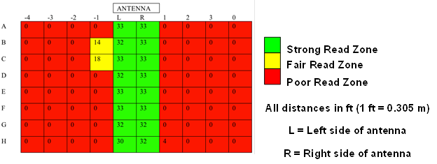
Figure 81. Diagram. Encapsulated single patch tag, linear polarization.

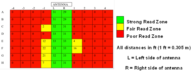
Figure 82. Diagram. Encapsulated single patch tag, circular polarization.

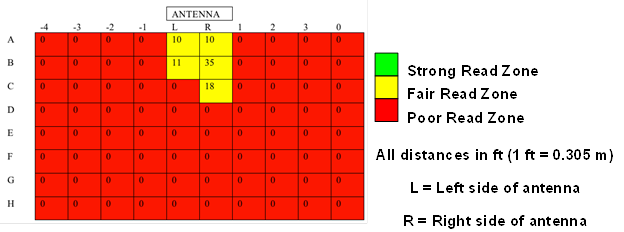
Figure 83. Diagram. Encapsulated monopole tag, linear polarization.

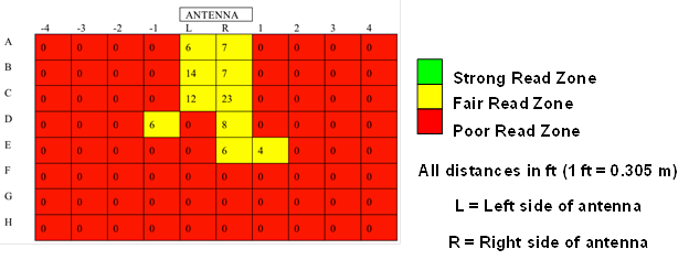
Figure 84. Diagram. Encapsulated monopole tag, circular polarization.

Encapsulated Tags Within Asphalt

In an effort to simulate survivability and readability under field conditions, the SAW tags were placed in HMA at about 392 °F (200 °C) and compacted in a gyratory compactor. All specimens were compacted at about 88 psi (600 kPa) pressure for 150 gyrations. Initially, unencapsulated patch and monopole tags were positioned in the gyratory specimens to evaluate their inherent survivability. Two of three unencapsulated tags were destroyed during compaction. Therefore, all subsequent tags evaluated in this read range study were encapsulated in thermally conductive epoxy.

The encapsulated tags were placed near the center of the gyratory plugs. As shown in figure 85, a variety of tag orientations were explored to determine which would provide the best readability. In addition to these orientations, the encapsulated tags were also rotated about the cylinder's axis to evaluate any further potential signal degradation. Figure 86 depicts the rotational positions of the asphalt sample.

Overall, the testing revealed that the strongest signal strength and readability were produced in orientation #1 (face side of the tag facing the antenna) for both the single patch and monopole tags. In this orientation, rotation #1 (figure 86) provided the best and most consistent results. Figure 87 and figure 88 summarize typical testing results for orientation #1 for both the monopole and single patch tags. Note that the single patch tag was read up to about 12 ft (3.6 m) from the antenna using this orientation. Although not shown, orientations #2 and #4 were also considered strong and reliable for both types of tags. In addition, the monopole tags performed well in orientations #4 and #6.

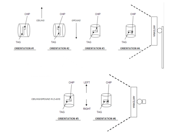
Figure 85. Drawing. Orientation guide for tags within asphalt specimens.

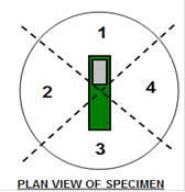
Figure 86. Drawing. Rotation scheme for tags within asphalt specimens (monopole and single patch).

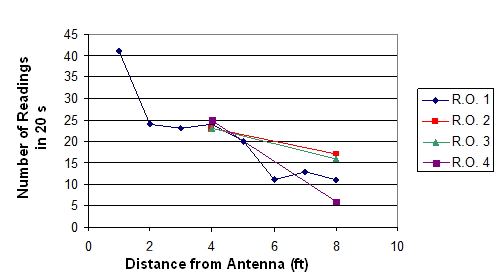
R.O. = rotational orientation
1 ft = 0.305 m
Figure 87. Graph. Orientation #1 for monopole tag using circular polarization.

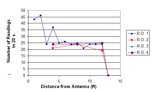
R.O. = rotational orientation
1 ft = 0.305 m
Figure 88. Graph. Orientation #1 for single patch tag using circular polarization.

Conclusions: Signal Strength and Readability

Overall, both the encapsulated monopole and patch antenna tags showed acceptable performance when encased in HMA. The monopole tags, while more practical and compact in size, did not perform as reliably as the patch tags in terms of signal strength and readability. Based on the entire laboratory read performance testing, both the monopole and patch tags warrant further investigation in field trials. Because they are to be pre-positioned ahead of the asphalt paver, they can be placed in the optimum location: orientation #1/rotational position #1.

Thermal Sensitivity

To simulate field conditions within a laboratory, the testing apparatus shown in figure 89 was developed for measuring the temperature sensitivity and transient response of the SAW RFID tags. As shown in the figure, the SAW RFID tags were pre-positioned on a flat wood plank covered in foil (to isolate temperatures and increase signal strength) and exposed to preheated materials. The selected materials used for testing included generically graded asphalt aggregate and HMA with about 5-percent binder content by weight. These materials were preheated to about 284 to 338 °F (140 to 170 °C) and placed over the test tag at room temperature. Upon exposure, tag temperatures were recorded over time via the RF SAW reader and software. Independent temperature measurements were collected using a Fluke® thermocouple probe affixed to the foil adjacent to the tag. Because our initial small supply of SAW RFID tags was limited, the tags tested here were the same as those used previously for the survivability and read performance testing; they were recovered from the gyratory plugs after completion of the survivability testing.

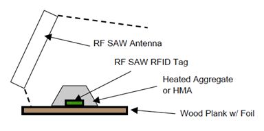
Figure 89. Drawing. Thermal testing apparatus.

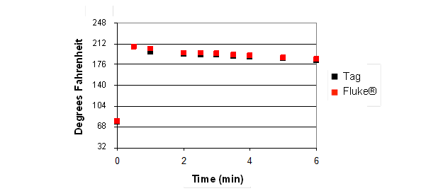
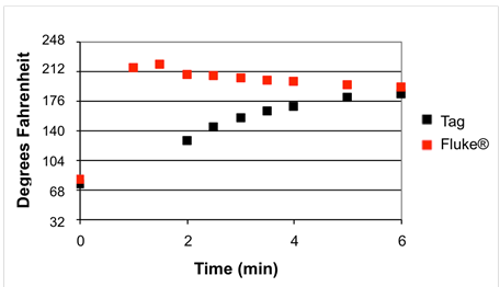
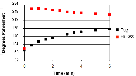
Table 17 describes the tags used for this study. figure 90 through figure 92 summarize the thermal sensitivity study results for hot aggregate material. Time zero corresponds to ambient (room temperature) conditions immediately before covering the RFID tag and Fluke® thermocouple with the hot aggregate. The test results show that the unencapsulated monopole tag (tag 0A21, figure 90) quickly matched the temperature readings from the thermocouple. The encapsulated monopole tag (tag 0443, figure 91) required about 5 to 6 min to reach aggregate temperature, as measured by the thermocouple. This thermal lag is assumed to be due to the additional thermal mass and relatively low thermal conductivity from the encapsulating epoxy. The thermal lag even more pronounced for the encapsulated patch tag (tag 09FE, figure 92) because of its larger format and corresponding larger mass of encapsulating epoxy. Even after 6 min, the encapsulated patch was 104 °F (40 °C) cooler than the reference measurement. Note that no unencapsulated patch tag was evaluated in this thermal study because it had been destroyed in the gyratory compactor during the first stage of the testing.

Table 17 . Tags employed in thermal testing.

°C = (°F - 32)/1.8
Figure 90. Graph. Thermal response from tag 0A21 using hot aggregate.

°C = (°F - 32)/1.8
Figure 91. Graph. Thermal response from tag 0443 using hot aggregate.

°C = (°F - 32)/1.8
Figure 92. Graph. Thermal response from tag 09FE using hot aggregate.

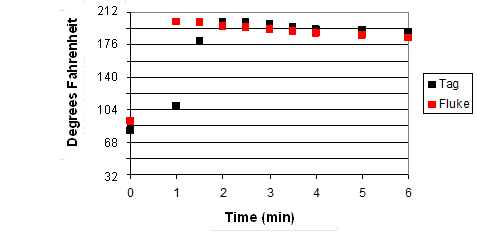
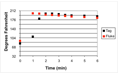
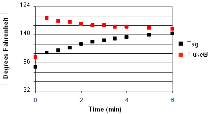
Figure 93 through figure 95 summarize the thermal sensitivity study results for the HMA material. Similar conclusions can be drawn here as for the hot aggregate: the unencapsulated monopole tag responds quickly and accurately, the encapsulated monopole tag responds with an acceptable time delay, and the encapsulated patch tag responds much more slowly and was still far from the equilibrium temperatures when the measurements ended at 6 min. This thermal lag may prove to be detrimental for field use.

Once the tags have equilibrated from the initial thermal shock (i.e., starting at ambient temperature and being covered with 284 to 338 °F (140 to 170 °C) HMA, they then match the thermocouple measurements for the continued slow cooling with time. This is most evident for the monopole tags (figure 93 and figure 94); readings were not continued for a long enough time period to completely confirm this for the encapsulated single patch tag (figure 95).

°C = (°F - 32)/1.8
Figure 93. Graph. Thermal response from tag 0A21 using hot HMA.

°C = (°F - 32)/1.8
Figure 94. Graph. Thermal response from tag 0443 using hot HMA.

°C = (°F - 32)/1.8
Figure 95. Graph. Thermal response from tag 09FE using hot HMA.

Overall, the thermal sensitivity study suggests that, given an adequate amount of time after HMA placement before compaction, all of the tested SAW RFID tags have transient thermal response sufficiently rapid for field use. The unencapsulated monopole tag performed more effectively than the others. Nonetheless, further field evaluation of all of the tags is justified.

FIELD EVALUATION

Field trials were conducted to evaluate the suitability of SAW RFID technology for wireless measurement of in-place HMA temperatures during intelligent compaction. These trials, hosted by MDSHA in conjunction with the FHWA Intelligent Compaction Pooled Fund Study, were conducted on July 23, 2009, during placement of a 1.5 inches (38 mm) pavement overlay.⁽¹³⁾

Site Information

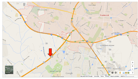
The project site for the field trials was located on United States Route 15/Maryland Route 340 in Frederick County, Maryland. More specifically, the site was located in the outer (right) northbound lane between Mt. Zion Road and the Jefferson Street Bridge. Figure 96 maps the general location of the project site.

Original image: ©2015 Google®; map annotations provided by University of Maryland
Figure 96. Map. Approximate location of project site.⁽²⁴⁾

Construction and activities related to the intelligent compaction field trial were conducted at the project site from about July 20 to July 24, 2009. An initial attempt was made on the evening of July 22 to perform the field evaluation of the SAW RFID temperature measurement system. However, all construction activities were cancelled because of an unexpected thunderstorm. The encapsulated tags for the field trial had already been affixed to the milled surface using epoxy putty before the storm. After cancellation, the tags were pried from the road surface and the epoxy putty was carefully ground off so that the tags could be reused on July 23. The field evaluation was completed on July 23 from about 0200 to 0300 h. Weather conditions were clear, mild, and windless. Table 18 summarizes weather data recorded just prior to testing from two nearby weather stations.

Table 18 . Weather data recorded near the project site for July 22-23, 2009.

Note: Walnut Ridge and Middletown stations are about 8 (12.88 km) and 36 mi (57.96 km), respectively, from the project site.
°C = (°F - 32)/1.8
1 mi/h = 1.61 km/h

Testing Procedure

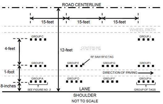
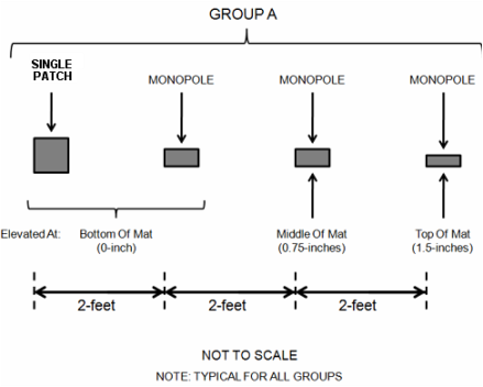
The test section was about 51 ft (15.5 m) long and was located near the interchange with Mt. Zion Road. Ten single patch tags and 30 monopole SAW RFID tags were pre-positioned ahead of the paver. In an effort to measure temperature through the depth of the overlay, three elevations were considered: bottom of the mat (elevation 0 inches), middle of the mat (elevation 0.75 inches (19 mm)), and surface of the mat (elevation 1.5 inches (38 mm)). The middle tags were elevated using a thicker layer of thermally conductive epoxy underneath the tag. Layout schematics for the test section are shown in figure 97 and figure 98.

1 ft = 0.305 m
Figure 97. Drawing. Plan view of test section.

1 ft = 0.305 m
1 inch = 25.4 mm
Figure 98. Drawing. Detailed plan view of a single group of SAW RFID tags.

As previously described, all of the tags except for eight "top of mat" surface tags were encapsulated in a relatively rigid thermally conductive epoxy. All tags other than those used for the surface were affixed to the milled existing pavement surface using quick-hardening epoxy putty (Loctite® 5-Minute Epoxy Putty). The mounted tags were oriented so that their ceramic chip and antenna were facing upward to enhance their readability. The unencapsulated surface tags were placed face down into the asphalt by the contractor immediately after passage of the paver. Figure 99 shows the tags being placed on the milled surface.

The RF SAW tag reader and circularly polarized antenna were mounted on a long-handled wheeled carriage to read the tags from the side of the road during compaction operations. The antenna was elevated about 1 ft (0.3 m) above the pavement surface. The wheeled apparatus was manually operated to minimize any disturbance to the hot asphalt or disruption of the compaction operations while the lift was cooling and being compacted. The reader was cabled to a laptop computer that recorded temperature and tag signal strength during testing.

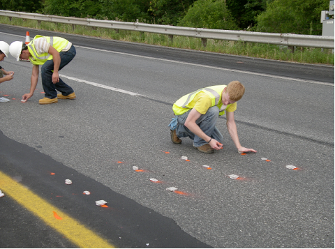
Figure 99. Photo. Placement of SAW RFID tags on surface of existing milled pavement.

The reader software requires that the operator specify a temperature window prior to reading the tags; the manufacturer recommends a 86 °F (30 °C) temperature window. This temperature window may be widened; however, the software signal processing time becomes longer. A longer signal processing time has been known to decrease the signal strength/response of the tag, especially when the tag is embedded in attenuating materials.

Thermal lag added another complication to obtaining good early temperature readings from the encapsulated tags immediately after they were covered with hot HMA. As described previously, thermal lag is the time required for the encapsulated tags to "heat up" to the temperature of the surrounding material. Results from the laboratory study suggested that the thermal lag for encapsulated tags is about 3 to 8 min, depending on the tag type; encapsulated single patch tags experience the longest thermal lag. The laboratory thermal sensitivity study also suggested that unencapsulated tags at the surface would exhibit only about 1 to 2 min of thermal lag.

The estimated temperature window immediately after placement of the overlay was set at 230 to 284 °F (110 to 140 °C). Initially, no response could be obtained from any tag. After the temperature window on the reader was adjusted downward to 176 to 230 °F (80 to 110 °C), some tags were read successfully at about 8 min after paving. The manufacturer-recommended temperature window of 86 °F (30 °C) was used throughout the field trials. However, during the initial heating of the tags (thermal lag) and rapid cooling of the mat immediately after placement, it proved difficult to adjust the temperature window on the reader quickly enough to capture the initial tag temperatures.

The wheeled reader and antenna apparatus was initially passed over the "Group A" tags (see figure 97 and figure 98), then "Group B," then "Group C," and so on, after which the cycle was repeated. The data collected during testing included the tag identification number, the time/date stamp of the last reading during the antenna pass, the tag distance from the antenna at the last reading, and the temperature at the last reading. Note that even if multiple reads were obtained from a tag during a given pass, the reader software saved only the data from the last read. Four full cycles of readings from Groups A through I were performed until the mat had cooled sufficiently that the vibratory compactors moved on to other sections. Prior to each pass, the reader software temperature window was adjusted for the decreasing temperature conditions. Figure 100 shows the paving operation and test setup during construction.

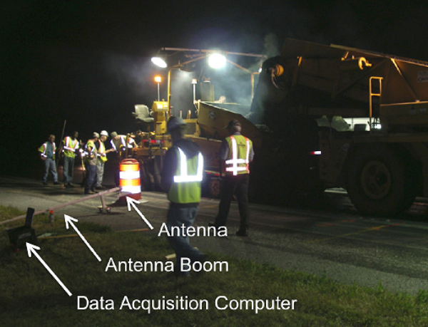
Figure 100. Photo. Paving operation and test setup during construction.

Field Test Results

After the hot-mix asphalt had been placed on the first groups of tags (Groups A through C), the vibratory compactors passed the testing area for a few minutes. Additional time was required to configure the reader software with a proper temperature window to read the tags. Consequently, the first tag reads were obtained about 8 min (± 1 min) after the tags were covered with asphalt. Readings were than taken for approximately the next hour, continuing after the vibratory compactors had moved on to subsequent sections of pavement.

Overall, the temperatures at the bottom of the mat decreased from 198 to 135 °F (92 to 57 °C) during the cooling period monitored in this study. At the middle of the mat and on the surface, temperatures generally decreased from 208 to 133 °F (98 to 56 °C) and from 219 to 111 °F (104  to 44 °C), respectively. Table 19 summarizes the read success rates for the tags. Five of the 30 preplaced tags could not be read successfully during system testing prior to paving operations. This is likely owing to damage caused by their removal from the roadway surface the night before and/or their preparation for reuse by grinding off the hardened epoxy putty. The read rates after asphalt placement and during compaction increased from 28 percent during the first pass to 52 percent in the fourth. This should not, however, be interpreted as an increase in the inherent read rate with time. Rather, this increase is because it was easier to set an appropriate temperature window in the reader software during the slower cooling of the later passes than during the rapid cooling in the first pass.

Table 19 . Tag read rates.

Evaluations of the cooling HMA temperatures with depth and time were performed at two transverse cross sections: Groups A-D-F-H and B-E-G-I. Results from cross section B-E-G-I are described here; the results from cross section A-D-F-H were very similar. Plots illustrating temperature versus time since paving are given in figure 101 through figure 103 for the bottom, mid-thickness, and surface of the mat, respectively. "Time since paving" is the estimated elapsed time after the tags are covered with the asphalt by the paver.

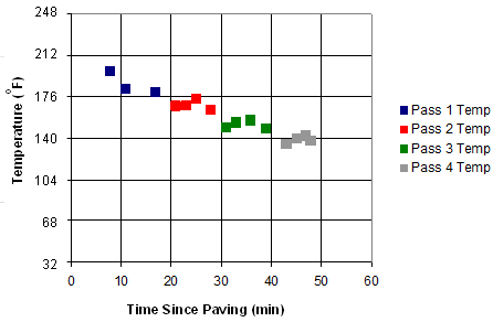
°C = (°F - 32)/1.8
Figure 101. Graph. Temperature versus time at bottom of mat (cross section B-E-G-I).

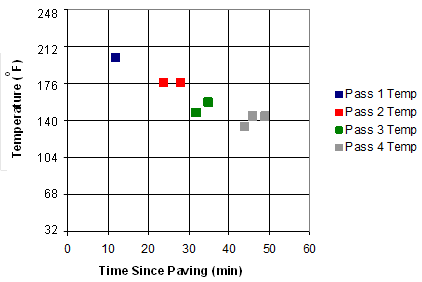
°C = (°F - 32)/1.8
Figure 102. Graph. Temperature versus time at middle of mat (cross section B-E-G-I).

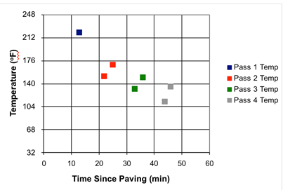
°C = (°F - 32)/1.8
Figure 103. Graph. Temperature versus time at surface of mat (cross section B-E-G-I).

As shown in the figures, the temperatures measured by the tags decreased with every compaction pass. Based on these test results and theoretical expectations for typical mat cooling trends, exponential regression lines were fit to the data. Figure 104 summarizes the cooling trends segregated by location within the mat thickness.

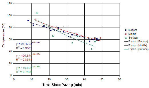
°F = (°C x 1.8) + 32
Figure 104. Graph. Temperature versus time segregated by location (cross section B-E-G-I).

The similarities between the regression lines shown on figure 104 are not suggestive of any systematic variations in temperature through the depth of the mat. This is likely because of the thinness of the overlay (1.5 inches (38 mm)) and other limitations of the test (inaccuracies in the depth of the tags and nonuniformity of initial paving temperatures). Therefore, all depth locations were combined, and a single exponential regression equation was fit to the combined dataset, as shown in figure 105.

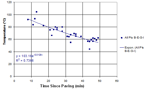
°F = (°C x 1.8) + 32
Figure 105. Graph. Temperature versus time averaged across depth (cross section B-E-G-I).

The exponential regression equation for the mat cooling at cross section B-E-G-I is shown in figure 106.

Figure 106. Equation. Exponential cooling equation at cross section B-E-G-I.

The corresponding regression equation for the mat cooling at cross section A-D-F-H is shown in figure 107:

Figure 107. Equation. Exponential cooling equation at cross section A-D-F-H.

These regression equations for the combined data are the basis for evaluating the traditional mat cooling models from the literature.

Variability and Reliability

In an effort to determine the reliability of the field test results and the consistency of the data collected, the following additional evaluations were made:

• Comparison of measured temperatures reported by single patch and monopole SAW RFID tags placed at the same location at the bottom of the mat.
  
  
• Comparisons of surface temperatures measured with the SAW RFID tags against independent measurements using a Fluke® infrared thermometer.
  
  
• Additional laboratory testing to determine the variability of temperature measurements from the SAW RFID tags based on errors generated by the reader.
  
  

These variability and reliability analyses were performed on the temperature data recorded from cross sections B-E-G-I and A-D-F-H.

To determine whether there were any systematic differences between the single patch and monopole tags, pairs of each were placed at the bottom of the mat approximately 2 ft (0.6 m) apart within each group (see figure 97 and figure 98). A comparison of the temperatures measured by each tag type is presented in figure 108, figure 109, and table 20.

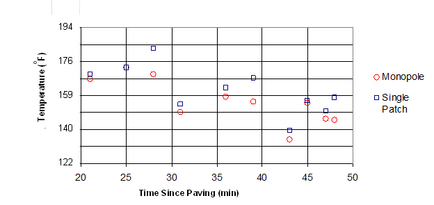
°C = (°F - 32)/1.8
Figure 108. Graph. Comparison of temperatures by tag type (cross section A-D-F-H, bottom of mat).

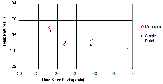
°C = (°F - 32)/1.8
Figure 109. Graph. Comparison of temperatures by tag type (cross section B-E-G-I, bottom of mat).

Table 20 . Temperature comparisons at bottom of mat.

- Indicates no data collected
°C = (°F - 32)/1.8

The maximum difference in temperature measured by the two types of tags at the bottom of the mat was about 9 percent for cross section A-D-F-H at 28, 39, and 48 min after paving. The average temperature difference for all of the tags was 4.6 percent at cross section A-D-F-H (standard deviation of 3.5 percent) and 3.7 percent at cross section B-E-G-I (standard deviation of 1.4 percent). These differing temperatures may be due to a general inaccuracy of the tags (possibly a systematic bias) or to spatial variability. However, on average, the temperatures were consistent within a 5-percent difference.

Comparisons were also made between surface temperatures measured using the SAW monopole RFID tags and independent measurements using a Fluke® infrared digital thermometer are summarized in figure 110 and table 21. More significant temperature variations are exhibited in this comparison; the maximum temperature difference was about 30 percent at 22 and 45 min and about 25 percent at 32 min. In addition, the difference is widely sporadic and inconsistent (ranging from approximately 7 to 30 percent). This may be the result of the different technologies between the Fluke® thermometer and the SAW RFID tags or spatial variability of the temperature distributions as the locations of the infrared readings were as much as several feet from the corresponding SAW RFID measurements. A more thorough explanation may require additional laboratory and/or field testing.

An additional laboratory study was performed to determine the inherent variability of the temperature measurements from the SAW RFID tags. The study was performed at constant room temperature. Repeated readings were taken to determine any fluctuating temperature readings caused by the SAW tags and reader rather than the environment. The result of the test found a negligible fluctuation of about ± 0.36 °F (± 0.2 °C). The manufacturer also states that transmission interferences (wireless communication and magnetic fields) may contribute to inaccuracies. However, this is unlikely to have been a major factor in the field trials.

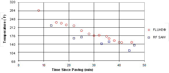
°C = (°F - 32)/1.8
Figure 110. Graph. Surface temperatures measured by SAW RFID tags versus Fluke® infrared thermometer.

Table 21 . Temperature comparisons at top of mat.

Conclusions: Field Evaluation

The overall findings from the field trials indicate that the SAW RFID tags can be used for measuring mat cooling temperatures during HMA construction. It is important, however, to understand that SAW RFID is still a developing technology-certain limitations and imperfections exist, but improvements in the technology are to be expected in the future. Specific conclusions related to various aspects of the field evaluation are described below.

Field Test Performance

• A temperature window must be specified in the RF SAW reader software to be able to read the in-place tags. This requirement may and did lead to operational issues in the field, particularly during the early stages of mat cooling when the temperature dropped rapidly, causing difficulty in setting the correct temperature window.
  
  
• The manufacturer recommends a 86 °F (30 °C) temperature window based on their calibration techniques at room temperature. The temperature window may be widened, but the software signal processing time then becomes longer and the signal strength/response of the tags decreases. The manufacturer's recommended temperature window of 86 °F (30 °C) was used for all of the field trials.
  
  
• There was difficulty differentiating physically damaged tags from those that simply could not be read immediately after paving/compaction. In other words, if a tag is nonresponsive to the reader, it might not be caused by destruction by vibratory compaction. It may be that the reader cannot get a response because the temperature window is incorrect or the tag signal is severely attenuated.
  
  

Field Test Results

• The field results generally show an exponential relationship between cooling temperatures and time. This generally agrees with theoretical considerations that suggest exponential cooling.
  
  
• No systematic temperature variations with depth were observed during mat cooling. In other words, the measured temperatures at the bottom, middle, and top of the asphalt mat, at any given location and time, were all within the variability range of the sensors. This may simply be a consequence of the thinness of the lift on this particular project.
  
  

Variability and Reliability

• Based on the comparative study at the bottom of the mat between the two types of tags (single patch and monopole) and previous laboratory testing, the temperatures recorded by the two tag types are reasonably consistent and accurate.
  
  
• The comparative study at the surface of the mat between the Fluke® infrared thermometer and monopole tag found inconsistencies between the two sets of readings. This may due to spatial variability. Additional field and/or laboratory testing are required for further explanation.
  
  

COMPARISONS BETWEEN PREDICTED AND MEASURED MAT COOLING

The mat cooling response measured using the SAW RFID tags is compared with the predicted temperatures versus time and depth from theoretical/numerical models. As will be described later, these comparisons require some field calibration of the model input parameters, given that there are no laboratory-measured values of the thermal properties for the mix placed at the field test site. The principal objectives of the comparisons between measured and predicted cooling response are the following:

• Determine whether the use of RFID technology to measure HMA cooling temperatures was accurate and successful.
  
  
• Identify improvements in the overall process of measuring mat cooling temperatures using RFID technology.
  
  
• Calibrate via a sensitivity analysis the values for the model input parameters that provide reasonable and close agreement with the field measured temperatures.
  
  

Analysis Inputs

The finite difference calculations for the analyses are based on figure 68 for the conduction calculations at the interior points and figure 72 for the heat balance at the mat surface. Table 22 summarizes the input parameter values used for the model predictions. These were selected based on recommendations from previous investigations and the results of the input parameter optimization presented later. Because the field construction was performed at night, the impacts of solar radiation (H_S) and absorptivity (α) are negligible. The convective heat transfer coefficient value corresponds to free convection at zero wind velocity. This is consistent with weather station data at the time of paving.

Table 22 . Input parameters used in models.

The depth and time increments for the finite difference calculations are summarized in table 23. Temperatures are calculated every 0.25 inches (6.4 mm) of depth through the 1.5-inch (38-mm) overlay and for an additional 6 inches (150 mm) into the underlying asphalt base. This is assumed to be a sufficient depth across which conductive heat flows are negligible over the duration of the analyses. The time step shown in figure 111 was selected to satisfy the stability requirement for the Euler time integration algorithm:

Figure 111. Equation. Stability requirement for Euler time integration algorithm.

The temperature at the lower boundary was fixed at 81 °F and the ambient air temperature was set at 71 °F. The initial conditions are a uniform 305 °F temperature for the HMA in the overlay and a uniform 81 °F temperature in the underlying base asphalt. The base asphalt and ambient air temperatures were measured during the field trials. The initial HMA temperature of the overlay was provided by MDSHA.

Table 23 . Input parameters used in finite difference solution.

Predicted Mat Cooling Response

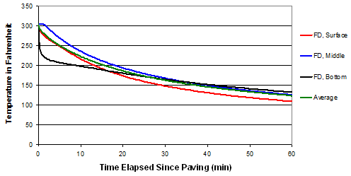
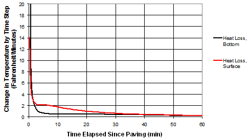
Figure 112 illustrates the predicted temperature versus time trends at the bottom, middle, and surface of the overlay and the average predicted temperature through the overlay thickness. As shown in the figure, the bottom of the mat expels the most heat initially, but as time elapses, the surface expels more heat than the bottom. These trends are consistent with those observed by Jordan and Thomas.⁽¹⁶⁾ Figure 113 displays these cooling trends more explicitly as changes in temperature per time step versus time. The temperature at the bottom of the mat initially drops more than 20 °F (11.2 °C) and then exponentially drops another 1 °F (0.56 °C) over the rest of the cooling process. The temperature of the surface of the mat initially drops about 13 °F (7.2 °C) and then, at about 2 min, begins to expel more heat than the bottom of the mat.

°C = (°F - 32)/1.8
Figure 112. Graph. Finite difference solutions for bottom, middle, and surface of mat.

°C = (°F - 32)/1.8
Figure 113. Graph. Cooling trends at the bottom and surface of the asphalt mat.

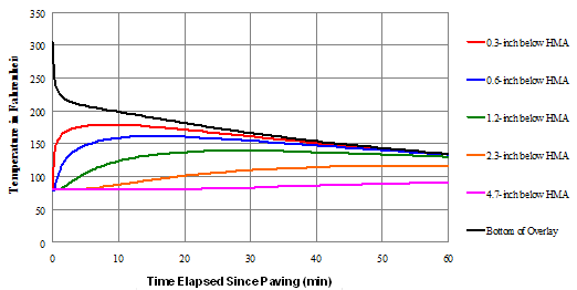
Figure 114 displays the temperature trends of the asphalt base as it heats and then cools as a result of conductive heat transfer from/to the HMA overlay. The asphalt base has an initial temperature of 81 °F and, upon placement of the hot HMA overlay, rapidly heats up via conduction. Over time, as the HMA overlay cools by convection and radiation, the heated base material cools along with the overlay. These cooling trends are logical and match physical expectations.

1 inch = 25.4 mm
°C = (°F - 32)/1.8
Figure 114. Graph. Base material temperatures cooling over time due to conductive heat transfer.

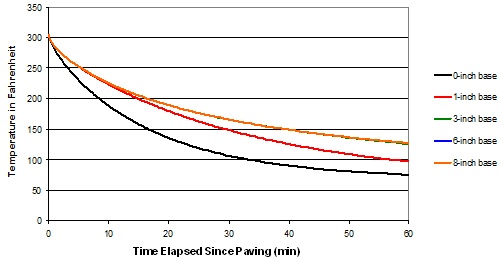
The decrease in temperature changes versus time at increasing depths within the base layer suggests that the arbitrary 6-inch (150-mm) depth for the lower fixed temperature boundary is sufficiently distant. As additional confirmation, figure 115 compares predicted cooling curves assuming base thicknesses of 0, 1, 3, 6, and 8 inches (0 25, 75, 150, and 200 mm). The cooling curves stabilize once the thickness of the base material exceeds 3 inches (75 mm).

1 inch = 25.4 mm
°C = (°F - 32)/1.8
Figure 115. Graph. Impact of lower boundary depth on average predicted temperature profile.

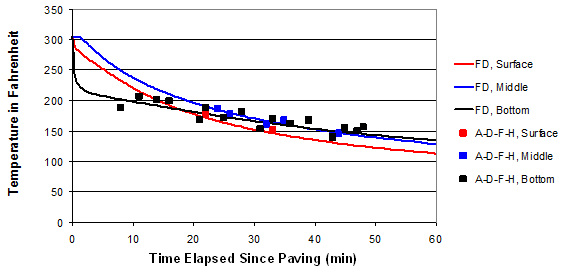
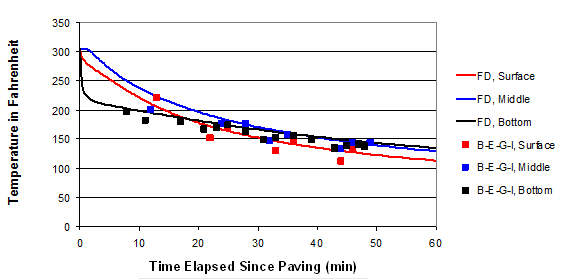
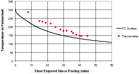
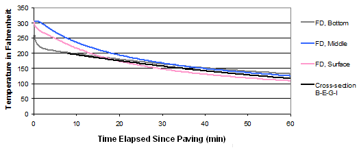
The results in figure 112 through figure 115 all suggest that the finite difference solutions are correct and a relatively accurate representation of field conditions. Figure 116 and figure 117 compare the calculated temperature trends at the surface, middle, and bottom of the mat with the corresponding measured data from cross sections A-D-F-H and B-E-G-I, respectively. As an additional check on accuracy of the predictions, Figure 118 compares the calculated temperatures at the surface against measured values obtained using the Fluke® infrared thermometer.

°C = (°F - 32)/1.8
Figure 116. Graph. Predicted versus measured temperatures at cross section A-D-F-H.

°C = (°F - 32)/1.8
Figure 117. Graph. Predicted versus measured temperatures at cross section B-E-G-I.

°C = (°F - 32)/1.8
Figure 118. Graph. Predicted versus measured surface temperatures.

The results in figure 116 and figure 117 show generally good agreement between measured and predicted temperatures over time. However, it is difficult to discern any systematic correlations between the calculated curves and the measured temperature values as a function of depth. This is most likely due to the thinness of the overlay and the imprecision in locating the RFID temperature sensors at specific depths. The comparison in figure 118 between the predicted temperatures at the surface and the measured values as obtained by the infrared thermometer are good in terms of trends, but the measured temperatures are consistently higher than the predicted values. This may indicate either errors in the finite difference predictions at the surface or, as described previously, inaccuracies in the infrared temperature measurements due to spatial variability.

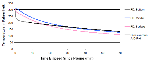
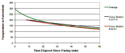
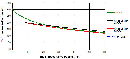
Because it was impossible to detect any systematic variations in measured temperatures through the depth, all depth locations were combined and fit with an exponential regression equation at each cross section as presented earlier in figure 106 and figure 107 for cross sections A-D-F-H and B-E-G-I, respectively. Figure 119 and figure 120 show the comparisons between the predicted temperatures and the exponential fits to the measured temperatures at the respective cross sections; figure 121shows the combined results from the two cross sections.

°C = (°F - 32)/1.8
Figure 119. Graph. Average measured versus predicted mat cooling at cross section  A-D-F-H.

°C = (°F - 32)/1.8
Figure 120. Graph. Average measured versus predicted mat cooling at cross section B-E-G-I.

°C = (°F - 32)/1.8
Figure 121. Graph. Average measured versus average predicted mat cooling.

The following observations can be made from the results in figure 119 through figure 121:

• The curvatures of the measured exponential curves are relatively close to the calculated curve, with the exception of the early portion of the response. However, in terms of temperature accuracy, the average curve and exponential curves begin to show a close correlation only after about 15 to 20 min after paving. The early-stage comparisons are complicated by the fact that the tags did not return any data until about 8 min after paving. Nonetheless, it seems clear that the tag and calculated temperatures are not consistent in trend and curvature during the early stages of cooling. Further field investigations may be required determine the causes for this inconsistency.
  
  
• Experience suggests that an average mat temperature of 175 °F (79 °C) is the threshold below which compaction is no longer economical or may even be injurious to the pavement (e.g., because of aggregate breakage). Therefore, temperature data from the time of initial paving to when it reaches 175 °F (79 °C) are considered the most valuable. Figure 122 superimposes the 175 °F (79 °C) line on the data from figure 122. The predicted and measured temperature data show close agreement only for about the last 5 to 10 min before the curves meeting the 175 °F (79 °C) threshold.
  
  

°C = (°F - 32)/1.8
Figure 122. Graph. Measured curves compared with calculated average curve with 175 °F line.

Conclusions: Comparisons Between Predicted and Measured Mat Cooling

The SAW RFID tags and equipment were successful in measuring the mat cooling temperatures during hot-mix asphalt placement. Comparisons with predictions from the finite difference computational models were generally favorable. However, there are inconsistencies between the predicted and measured temperatures, particularly during the early stages of the cooling response that may be due to limitations in technology, operator error, modeling error, or other causes. Further study is recommended to investigate and/or address the following:

• Recording temperature data immediately after paving rather than a few minutes afterward. This may be accomplished by preheating the tags to the initial asphalt temperature. The RF SAW reader software can then be adjusted more easily to read the tags immediately after paving.
  
  
• Improvement in the RF SAW reader and software to eliminate the need to set a temperature window.
  
  
• Performance of more field trials that incorporate traditional temperature measuring instrumentation (e.g., thermocouples). Comparing the SAW RFID with the traditional instrumentation should identify any limitations or inaccuracies in the SAW RFID technology in this application.
  
  
• Determine an encapsulation method and material that optimizes the functionality of the tag in terms of readability, thermal response, and physical survivability.
  
  

SENSITIVITY ANALYSIS AND CALIBRATION TECHNIQUES

No laboratory tests to determine the input parameter values for the mat cooling model were performed in this study. Instead, typical initial estimates of the input parameter values were obtained from the literature. However, these values varied widely among the citations, and the appropriateness of some of the recommended values was suspect. A series of sensitivity and calibration analyses were therefore performed to determine better values for the model input parameters to use in the numerical simulations described in the preceding section. These analyses provided additional confidence and validation that the numerical solutions are logical and correct as well as producing field-calibrated values for the inputs. The following subsections detail sensitivity analyses for the following inputs: thermal diffusivity and thermal conductivity, convective heat transfer coefficient, and emissivity. A calibration procedure to determine the input parameter values that produce the best fit between the measured and calculated temperatures is also described. This field calibration technique enables accurate predictions from the mat cooling model in the absence of laboratory measured input parameters.

Thermal Diffusivity and Conductivity

As described earlier, Luca and Mrawira conducted laboratory experiments to identify thermal properties for Superpave mixtures.⁽²¹⁾ They measured thermal diffusivity α and thermal conductivity k and compared their measured values with ranges cited in the literature (table 15 and table 16, respectively).

The sensitivity analyses aim to determine how changes in thermal diffusivity and conduction affect the curvature, rate of cooling, and other characteristics of the predicted cooling response. Note that changes in thermal diffusivity also imply changes in the analysis time step to satisfy the stability requirement for the Euler time-integration algorithm as given by figure 111.

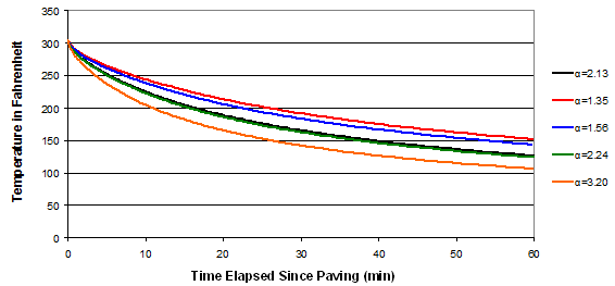
As shown in table 15, Luca and Mrawira found that thermal diffusivity may range from 1.35x10^-2 to 3.20x10^-2 ft²/h (1.25x10^-3 to 2.98x10^-3 m²/h). Five sample values within this range were therefore selected for the sensitivity analysis: 1.35 x10^-2, 1.56 x10^-2, 2.13 x10^-2, 2.24 x10^-2, and 3.20 x10^-2 ft²/h (1.25x10^-3, 1.45x10^-3, 1.98x10^-3, 2.08x10^-3, and 2.98x10^-3 m²/h). Similarly, Luca and Mrawira found that thermal conductivity may range from 0.58 to 2.24 BTU/ft-h-°F (1.0 to 3.9 W/m-°K) (table 16). Four sampled values within this range were therefore selected for the sensitivity analysis: 0.58, 0.64, 1.01, 1.19, and 2.24 BTU/ft-h-°F (1.00, 1.11, 1.75, 2.06, and 3.88 W/m-°K). Luca and Mrawira emphasized that thermal diffusivity and conductivity are generally difficult to predict and measure. Therefore, parameter values that fall outside the ranges in table 15 and table 16 should not be considered infeasible.

Figure 123 and figure 124 illustrate the results of the sensitivity analyses for thermal diffusivity and conductivity. Changing either the thermal diffusivity or the thermal conductivity values significantly affects the curvature and rate of cooling of the predicted mat cooling response. When interpreting the results in figure 123 and figure 124, it is important to remember that thermal diffusivity and conductivity are interrelated (see figure 65). Figure 123 shows that the rate of cooling increases with increasing thermal diffusivity. This is sensible; from figure 65, increasing α at constant k implies a decreasing specific heat capacity C_p, i.e., decreasing thermal inertia, hence a faster cooling rate. Figure 124 shows that the rate of cooling decreases with increasing thermal conductivity. At first glance, this appears paradoxical, because one would intuitively expect that an increased ability to conduct heat would lead to faster cooling. However, the observed behavior is indeed sensible given the relationship in figure 65: increasing k at constant α implies increasing specific heat capacity, i.e., increasing thermal inertia, hence a slower cooling rate.

k = 0.64 BTU/ft-h-°F (1.10W/m-°K)
°C = (°F - 32)/1.8
Figure 123. Graph. Sensitivity analysis for thermal diffusivity.

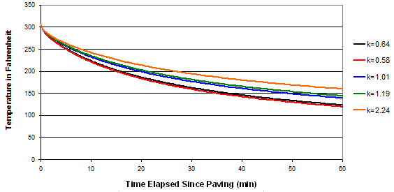
α= 2.13x10^-2 ft²/h (1.98x10^-3 m²/h)
°C = (°F - 32)/1.8
Figure 124. Graph. Sensitivity analysis for thermal conductivity.

Convective Heat Transfer Coefficient

Wolfe and Colony developed a relation for estimating convective heat transfer coefficients for an open highway construction environment that considered both free and forced convection principles.^(17,18) After studying various methods for estimating the convective heat transfer coefficient h, Wolfe, Heath, and Colony recommended the relation in figure 73.⁽¹⁹⁾

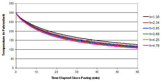
The sensitivity analysis for the convective heat transfer coefficient aims to determine how changes in convection affect the curvature, rate of cooling, and other characteristics of the predicted cooling response. Table 24 displays a series of increasing wind velocities and their correlating value for the convective heat transfer coefficient when using the equation in figure 73. These convective heat transfer coefficients are used as input parameters for the sensitivity analysis. Figure 125 illustrates the results.

Table 24 . Comparison of convective heat transfer coefficients.

°C = (°F - 32)/1.8
Figure 125. Graph. Sensitivity analysis for the convective heat transfer coefficient.

Based on the results in figure 125, altering the convective heat transfer coefficient does affect the curvature and rate of cooling of the mat cooling model. However, it is less pronounced than in the case of thermal diffusivity (figure 123) or thermal conductivity (figure 124). As the convective heat transfer coefficient increases, the curvature and rate of cooling increases. This is sensible; an increasing convective heat transfer coefficient means that more heat is lost through the surface, which, in turn, will cause the mat to cool more quickly.

Emissivity

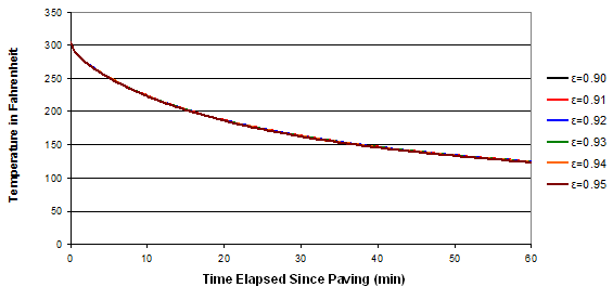
Emissivity is the pavement surface's relative ability to emit heat energy via radiation. It is defined as the ratio of the actual heat energy radiated by the pavement to the heat energy radiated by an idealized object that emits all radiation at the given temperature, i.e., a "perfect radiator."⁽¹⁵⁾ Wolfe and Colony recommend a relatively narrow range of 0.90 to 0.95 for the emissivity of an asphalt surface.⁽¹⁷⁾ Therefore, a sensitivity analysis comparing values 0.90 through 0.95 was performed to determine its effect on the curvature, rate of cooling, and other characteristics of the predicted temperature response. The results displayed in figure 126 suggest that altering the input value for emissivity has little impact on the curvature and rate of cooling of the predicted cooling response.

°C = (°F - 32)/1.8
Figure 126. Graph. Sensitivity analysis for emissivity.

Input Parameter Optimization Via Calibration

An optimization was performed on the input parameters using Microsoft® Excel Solver to determine the input values providing the best agreement between the measured and calculated temperatures. Based on the literature, it is known that the input parameters (thermal diffusivity, thermal conductivity, convective heat transfer coefficient, and emissivity) are not easily predicted or measured. Determination of these values through a field calibration process may expedite use of the mat cooling models by eliminating the need for laboratory testing to determine the input parameters.

To perform the optimization, the predicted temperatures from the mat cooling model are compared with the actual field-measured temperatures. The sum of the squared residual values between the predicted and measured temperatures is minimized in the Microsoft® Excel Solver tool by changing the input parameters for thermal diffusivity, thermal conductivity, convective heat transfer coefficient, and emissivity. Constraints are set within Solver to prevent negative values.

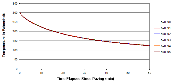
Two optimizations were performed: one that held the convective heat transfer coefficient h constant at 1.3 (figure 73 for the negligible wind speed observed in the field) and one that also optimizes h. Table 25 and table 26 summarize the results from both optimizations. Figure 127 compares the predicted cooling curves using the input values from the two optimizations. Both sets of optimized input parameters produce identical calculated average cooling curves. Therefore, based on the sensitivity analysis and recommendations from the literature, the selected input parameters used in this study have been taken from table 25, with the value of the convective heat transfer coefficient as recommended by Wolfe, Heath, and Colony.⁽¹⁹⁾ However, table 26 would have equally sufficed.

°C = (°F - 32)/1.8
Figure 127. Graph. Comparing both sets of optimized input parameters for the mat cooling model.

Table 25 . Results of Optimization #1-h constant.

Table 26 . Results of Optimization #2-h optimized.

These successful optimizations demonstrate that it is possible to field-calibrate thermal diffusivity, thermal conductivity, convective heat transfer coefficient, and emissivity. For a specific paving construction project, these input parameters can be determined by field calibration to limited field temperature measurements at the beginning of the project, eliminating the need for complex laboratory testing.

Conclusions: Sensitivity Analysis and Calibration Techniques

Each of the major input parameters was analyzed for its individual impact on the predicted cooling response. These sensitivity analyses provide added confidence that the numerical solutions are logical and correct. The following results were obtained:

• Thermal diffusivity: Based on the results shown in figure 123, altering the thermal diffusivity significantly affects the curvature and rate of cooling of the predicted response. As the value for thermal diffusivity increases, the curvature and rate of cooling increases.
  
  
• Thermal conductivity: Based on figure 124, altering the thermal conductivity significantly affects the curvature and rate of cooling of the model. As the value for thermal conductivity increases, the curvature and rate of cooling decreases.
  
  
• Convective heat transfer coefficient: Based on the results shown in figure 125, altering the convective heat transfer coefficient affects the curvature and rate of cooling of the mat cooling model. As the value for the convective heat transfer coefficient increases, the curvature and rate of cooling increases.
  
  
• Emissivity: Based on the results shown in figure 126, altering the emissivity has little impact on the curvature and rate of cooling of the mat cooling model.
  
  

A field calibration procedure using the Microsoft® Excel Solver tool successfully determined the optimum input parameter values for this study. For a specific paving construction project, the thermal diffusivity, thermal conductivity, convective heat transfer coefficient, and emissivity values may be determined by calibration to limited field temperature measurements at the beginning of the project, eliminating the need for complex laboratory testing.

OVERALL CONCLUSIONS AND LESSONS LEARNED REGARDING TEMPERATURE MEASUREMENT

The overall purpose of this study was to evaluate RFID-based wireless temperature sensors and traditional asphalt mat cooling models to predict temperature versus depth and time to better interpret stiffness feedback data from intelligent compactors. This work was done in conjunction with the FHWA Pooled Fund Study on Intelligent Compaction.⁽²⁵⁾ More specifically, the objectives are as follows:

• Evaluate the feasibility of using SAW-based RFID technology to measure HMA temperatures via wireless sensors.
  
  
• Demonstrate, in the field, the survivability and temperature measurement capabilities of the SAW RFID sensors during a pavement overlay.
  
  
• Consolidate data to develop asphalt cooling curves of measured temperature versus time.
  
  
• Compare measured cooling response with predictions from theoretical mat cooling models.
  
  
• Perform a sensitivity analysis of the effect of relevant input parameters in the theoretical mat cooling models on the predicted cooling response. From the sensitivity analysis, explore field-calibration techniques to expedite the use of the mat cooling models without requiring laboratory measured input parameters.
  
  

Based on the evaluations and experiments performed in this thesis, the following conclusions were reached regarding the above-mentioned objectives:

Laboratory Evaluation

Through laboratory analysis and information from the literature, an encapsulation process was developed to protect the SAW RFID tags from physical damage (during construction) while promoting heat transfer. It is recommended that additional work be performed to determine the minimum thickness of the epoxy coating to optimize tag readability while ensuring survivability.

In terms of signal strength and readability, both the encapsulated monopole and patch antenna tags showed acceptable performance when encased in HMA specimens. The monopole tags, while more practical and compact in size, do not perform as reliably as the patch tags in terms of signal strength and readability. Both tags performed the best when aligned closely to "orientation #1/rotation #1" (see figure 85 and figure 86). Regarding thermal response, a thermal lag was observed after exposing the encapsulated tags to hot material. This lag is defined as the time required for the tag to "heat up" to match its environment. The encapsulated single patch tags required the longest thermal lag of about 5 min.

Field Evaluation

Overall, the findings from the field evaluation were that the RF SAW RFID tags can measure asphalt mat cooling temperatures during paving and compaction. It is important to note SAW RFID is a developing technology-certain constraints and imperfections exist, and improvements in the technology are expected in the future. The following subsections summarize the conclusions from the field evaluation in terms of field test performance, field test results, and variability and reliability:

Field Test Performance

The RF SAW tag reader requires a narrow temperature window to read the in-place tags. This requirement led to operational issues in the field, especially during the early stages of the asphalt cooling when temperatures dropped rapidly. The manufacturer recommends a 86 °F (30 °C) temperature window based on their calibration techniques at room temperature. It is recommended that additional future field tests be performed to more closely monitor the initial temperature of the HMA, perhaps by preheating the tags so that they can be read immediately after paving. Alternatively, the manufacturer of the SAW RFID technology could eliminate the use of a temperature window from the reader software.

There was also difficulty differentiating permanently damaged tags from those that simply could not be read immediately after paving/compaction. In other words, if a tag is nonresponsive to the RF SAW reader, it might not be caused by destruction due to high temperatures or vibratory compaction. It may be that the reader cannot get a response because the temperature window is incorrect or the tag's signal is severely attenuated.

Field Test Results

The field results generally show an exponential relationship between cooling temperatures and time. This generally agrees with theoretical considerations that suggest exponential cooling. No systematic temperature variations with depth were observed during mat cooling. In other words, the measured temperatures at the bottom, middle, and top of the asphalt mat, at any given location and time, were all within the variability range of the sensors. This may simply be a consequence of the thinness of the lift on this particular project.

Variability and Reliability

Based on the comparative study at the bottom of the mat between two sets of tags (single patch and monopole) and previous laboratory testing, the temperatures recorded by the two tag types are reasonably consistent and accurate. The comparative study at the surface of the mat between the Fluke® infrared thermometer and monopole tag found larger inconsistencies between the two sets of readings. This may be the result of testing at different locations on the mat surface. Additional field and/or laboratory testing are recommended to resolve this issue.

Comparisons Between Measured and Predicted Mat Cooling Response

RF SAW RFID tags and equipment can be used for measuring the mat cooling temperatures during hot-mix asphalt placement. Predicted temperatures from the theoretical heat transfer model (using input parameters obtained from the literature and through field calibration) agreed with field measurements. However, there are inconsistencies between the two that may either be due to limitations in the technology or to operator error. Further testing is recommended to investigate and remediate the following:

• Recording temperature data immediately after paving rather than a few minutes afterward. This may be accomplished by preheating the tags to the initial asphalt temperature-during laboratory testing, the tags exhibit a thermal lag in meeting their intended temperature. The RF SAW reader software can then be adjusted to read the tags accordingly; or simply improved by the manufacturer.
  
  
• Incorporating traditional thermocouple temperature sensors that have been used successfully in the past. Comparing the SAW RFID with the traditional equipment can better identify any limitations in the SAW RFID technology for this application.
  
  
• Refining the encapsulation process to optimize readability and survivability. During the field trials, there was difficulty differentiating physically damaged tags from those that simply could not be read immediately after paving/compaction. In other words, if a tag is nonresponsive to the reader, it might not be caused by destruction by vibratory compaction. It may be that the reader cannot get a response because the temperature window is incorrect or the tag's signal is severely attenuated.
  
  

Sensitivity Analysis and Calibration Techniques

Sensitivity analyses were performed on key input parameters, and a field calibration procedure was developed to optimize the accuracy of the theoretical cooling response predictions. The following conclusions were drawn from these analyses:

• Increasing thermal diffusivity increases the curvature of the cooling curve and the rate of cooling.
  
  
• Increasing thermal conductivity reduces the curvature of the cooling curve and the rate of cooling.
  
  
• Increasing the convective heat transfer coefficient increases the curvature of the cooling curve and the rate of cooling.
  
  
• Emissivity has little impact on the predicted cooling response.
  
  
• The input parameter values for this study were determined through a field calibration process. Microsoft® Excel Solver can be used to optimize the thermal diffusivity, thermal conductivity, convective heat transfer coefficient, and emissivity values to minimize the discrepancies between predicted and measured temperatures. For any specific paving construction project, these input parameters can be determined by field calibration to limited field temperature measurements at the beginning of the project, eliminating the need for complex laboratory testing.
  
  

Lessons Learned

Based on the experiences and results of this study, the following lessons were learned:

• The encapsulation of the tags should be uniformly and minimally thin. In this study, the thickness of the encapsulant for each tag varied slightly, causing variability in the laboratory and field test results.
  
  
• To determine whether there is the possibility of systematic variation within a pavement layer, future testing should be performed on thicker pavement overlays. It was difficult to discern systematic variations in temperature versus depth for the very thin 1.5-inch (38-mm) overlay examined in this study.
  
  
• Future field trials should be performed under daytime conditions so that the solar absorption terms in the mat cooling models can be exercised and evaluated.