U.S. Department of Transportation
Federal Highway Administration
1200 New Jersey Avenue, SE
Washington, DC 20590
202-366-4000
Federal Highway Administration Research and Technology
Coordinating, Developing, and Delivering Highway Transportation Innovations
| REPORT |
| This report is an archived publication and may contain dated technical, contact, and link information |
|
| Publication Number: FHWA-HRT-15-019 Date: May 2015 |
Publication Number: FHWA-HRT-15-019 Date: May 2015 |
Initial evaluations of the MERRA data presented in the previous chapter suggest that they are as good as, and in many ways superior to, weather data time series from conventional surface-based OWSs. The recommendations from these initial evaluations were that LTPP should adopt MERRA as the data source for its next update to the climate data module and develop a tool to extract and use these data for engineering applications.
These recommendations were presented as a draft phase 2 report that was subsequently reviewed by the Transportation Research Board’s ETG on LTPP Special Activities, FHWA experts, and LTPP staff.(1) The project team received and addressed 118 comments on the draft phase 2 report. Two primary comments necessitate additional analysis
with the following primary objectives:
This chapter addresses the first of these objectives. It can be broken down into the following set of specific study activities:
A variety of data sources were examined in this study. Ground-based climate data provided as part of the MEPDG serve as the standard input for flexible and rigid pavement simulations using the Pavement ME Design® software. Additional data sources employed for comparisons with the MEPDG climate files include the USCRN, the NWS Cooperative Observer Program (COOP), the Department of Energy Solar Infrared Radiation System (SIRS), and NASA’s MERRA. Further details on MEPDG, USCRN, COOP, SIRS, and MERRA are provided below.
The MEPDG methodology is implemented in the Pavement ME Design® software product from AASHTO. The climate data files needed as inputs to the MEPDG methodology and supplied with the Pavement ME Design® software are derived from two data products provided by the NCDC: the ULCD for times prior to 1 January 2005 and the QCLCD for times after 1 January 2005. Many of the ULCD and QCLCD sites are part of the NWS ASOS. Despite the limited QC incorporated in the QCLCD product and additional QC measures undertaken by the MEPDG model developers, these reference inputs still contain numerous measurement and/or data processing errors. However, a nonexhaustive review of the data found that the edited QCLCD data after 1 January 1, 2005, contains fewer processing errors than the unedited ULCD data prior to January 1, 2005. The QCLCD product includes hourly meteorological measurements for approximately 1,600 stations located across the United States.
The MEPDG climate data are the inputs to the EICM. The developers of MEPDG performed additional QC steps on the ULCD and QCLCD products for use with the EICM. Nonetheless, the climate data provided with the MEPDG still contain some measurement and data coding errors and time series gaps, albeit reduced as a result of the additional quality control steps.
Table 12 summarizes the meteorological data evaluated in this study, both from the MEDPG climate files and from the other climate data sources described in the subsequent sections.
Table 12. Variables employed from each measurement product for use during analysis.
| Variable of Interest | QCLCD |
MEPDG |
USCRN |
MERRA |
COOP |
SIRS |
| Air Temperature | X |
X |
X |
X |
X4 |
— |
| Dew Point Temperature1 | — |
— |
— |
— |
X5 |
— |
| Specific Humidity1 | X |
X |
X |
X |
— |
— |
| Wind Speed | X |
X |
— |
X |
X5 |
— |
| Precipitation | X |
X |
X |
X |
X5 |
— |
| Shortwave Radiation | — |
— |
X |
X |
— |
X |
| Cloud Cover Fraction2 | — |
X |
— |
X |
— |
— |
| Sky Condition3 | X |
— |
— |
— |
— |
— |
| 1Dew point temperature and specific humidity provide equivalent information regarding humidity 2Cloud cover fraction serves as a proxy for shortwave radiation 3Sky condition serves as a proxy for cloud cover fraction, and hence, shortwave radiation 4Only daily maximum / minimum / average values are available to the public 5Only daily average values are available to the public X = measurement/estimate is available at the majority of locations — = Data not included in source QCLCD = Quality Controlled Local Climatological Data MEPDG = Mechanistic Empirical USCRN = United States Climate Reference Network MERRA = Modern-Era Retrospective Analysis for Research and Application COOP = Cooperative Observer Program SIRS = Solar Infrared Radiation System |
||||||
USCRN
A summary describing the USCRN was provided in chapter 3. Observations collected by the USCRN were of particular interest in this study because they are derived from a minimum of three clustered sensors that are then averaged together prior to public distribution. The averaging of multiple measurements at each point in time serves to reduce measurement error and hence provides what is arguably the closest estimate of the ground truth. It is worth emphasizing here that all measurements inherently contain error. In addition, weather data are spatially variable, and measurements separated by even only a few hundred meters will be slightly different. However, for purposes of this study the USCRN measurements were considered as “reference” measurements of the true value of the meteorological data at the site.
Daily measurements of meteorological variables are available through the NWS COOP. COOP measurements collected from more than 570 individual station locations, were employed for use in this study. As opposed to the hourly (or shorter) measurements collected for the data products outlined in the preceding sections, COOP only provides daily averages and the daily range (i.e., maximum and minimum values) for certain meteorological variables. As a result, COOP data were used in this study to examine more closely the diurnal range of values from the hourly products in table 12 and to provide further insights regarding the fidelity of the different hourly products.
Ground-based radiometer measurements from the SIRS program operated by the Atmospheric Radiation Measurement Program under the auspices of the United States Department of Energy were used for direct comparison against model estimates of shortwave radiation.(67) Only the USCRN and MERRA products contain estimates of downwelling shortwave radiation at the surface. MEPDG estimates of downwelling shortwave radiation are inferred from cloud cover conditions (fraction) by employing an empirical expression described later in this report. Using this approach, it was possible to compare different solar radiation estimates even though not all of the data products contained direct estimates of downwelling shortwave radiation at the surface.
Meteorological inputs used to force the model were obtained from the MERRA product (http://gmao.gsfc.nasa.gov/merra/).(45) MERRA is provided at an hourly temporal resolution, 0.5by 0.67 degrees (latitude/longitude) spatial resolution, and is available from 1979 to the present. Chapter 4 provides a summary description of MERRA.
The MERRA product results from the merger of a physically based model (i.e., the NASA GEOS-5 Version 5.2.0) with satellite, airborne, ship, and radiosonde observations of the atmosphere. NASA frequently uses the MERRA product to help verify seasonal climate forecasting systems, generate climate data records, serve as input to satellite retrieval algorithms, and provide atmospheric forcings for hydrologic and land surface process studies.(49) In addition, MERRA is regularly analyzed and validated to ensure continuity and consistency because the data product is produced in near real-time.
A major advantage of MERRA over ground-based climate data sources is the uniform spatial coverage. The ground-based ASOS stations that provide much of the MEPDG/ULCD/QCLCD climate data are mostly located at airports and therefore clustered along the east and west coasts of the United States and around major population centers.
Measurement Product Collocation
To compare measurements from one measurement network against those from another, it is first necessary to collocate the measurement networks in space prior to collocating the measurement sequences in time. The collocation process was conducted for the QCLCD station locations (and hence the MEPDG station locations by association). That is, all computed distances treat the given QCLCD station as located at the center of the search area. Next, for a given QCLDC station, the horizontal distance was computed for every station in each of the measurement networks outlined above. A minimum separation distance of 0.5 degrees (approximately 31.1 mi at mid-latitudes) was specified. This was done so that each collocated set of measurement stations would be representative of the same local topographic and climate conditions. In addition, given the spatial resolution of the MERRA product, this guaranteed that at least one MERRA location (grid cell) would correspond to every QCLCD (and hence every MEPDG) station location. If at least one station location from each of the measurement networks outlined above was within 0.5 degrees of the given QCLCD measurement station, then those respective measurement stations from each measurement network were used during the statistical analysis discussed later.
Figure 62 through figure 64 show the histograms of the horizontal separation distances from the collocation procedure. As illustrated in figure 62, the MEPDG weather stations are derived directly from the QCLCD data set, and hence the separation distance is often equal to zero. Because there are many more QCLCD stations than MEPDG stations, sometimes more than one QCLCD station falls within the spatial threshold available for comparing against a given MEPDG station—this results in the occasional nonzero separation distances between QCLCD and MEPDG station locations. The MERRA data, as expected, showed the greatest range in separation distance (see figure 64).
Figure 65 shows the locations within the contiguous United States of the various climate data products examined in this study. A total of 354 combinations of USCRN, QCLCD, and MERRA data sites (diamond symbol) were collocated to within 0.5 degrees of horizontal separation.
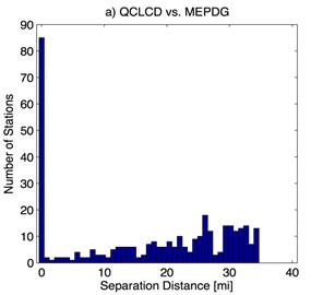
Figure 62. Histogram. Histogram of separation distances (in mi) relative to QCLCD for MEPDG stations.
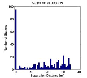
Figure 63. Histogram. Histogram of separation distances (in mi) relative to QCLCD for USCRN stations.
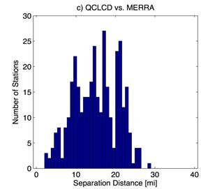
Figure 64. Histogram. Histogram of separation distances (in mi) relative to QCLCD for MERRA grid points.
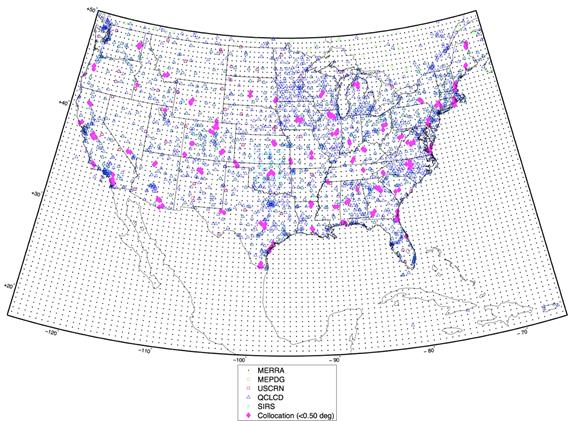
Figure 65. Map. Collocated USCRN, QCLCD, and MERRA data sets.
Elevation and Temperature Correction
Discrepancies in measurement elevation arise because not all collocated measurement locations are at precisely the same location in space. These discrepancies are greatest in regions of complex terrain (e.g., Rocky Mountains) and are less apparent in regions of low topographic relief. Because elevation differences can cause differences in air temperature, an air temperature correction was implemented to remove any systematic biases associated with elevation differences. The process was implemented in the MERRA product; it was not deemed necessary in the ground-based measurement products because most of the ground-based measurement stations are located in relatively flat terrain (e.g., at airports).
If differences exist between the land surface elevation at the MERRA grid point and the ground-based meteorological station, the MERRA air temperature is adjusted using an adiabatic lapse rate. If the elevation difference is positive (i.e., the ground station elevation is greater than the MERRA elevation), the ambient lapse rate is assumed to equal -8.0 °K/km. Conversely, if the elevation difference is negative (i.e., the station elevation is less than the MERRA elevation), the ambient lapse rate is assumed to equal -6.5 °K/km.(59) The difference between the two lapse rates accounts for the possibility of condensation during adiabatic cooling. Using the appropriate lapse rate, γ the temperature correction is then computed as shown in figure 66:

Figure 66. Equation. Adiabatic lapse rate temperature correction equation
Where Δ z is the elevation difference between the ground station and the nearest MERRA grid point and is defined as positive in the upward direction. Adiabatic air temperature adjustments were typically small (less than 1 °K) because the majority of locations used in this study had elevation differences less than 328 ft. However, a few study locations in complex terrain contained elevation differences upwards of 1,640 ft, which could result in temperature adjustments as large as 4 °K.
Statistical Comparisons of Data Sources
Statistical analyses were conducted between the different data sources relative to USCRN (i.e., USCRN treated as the reference measurement) for the approximately 17-year period of July 1, 1996, through September 1, 2013. This time period corresponds to the approximate temporal overlap of all of the available data sources used in this study. The emphasis of the statistical evaluation was on temperatures because prior studies had shown that pavement performance was most sensitive to these climate inputs.(1,2) Wind speed and cloud cover are the next most sensitive climate inputs; however, the USCRN data do not contain these data elements, and consequently, they could not be evaluated. Although the MEPDG in its current form assumes no infiltration of surface water into the pavement layers, precipitation data from the various climate data products were nevertheless compared. Cloud cover, wind speed, and humidity were also compared to a lesser extent. Cloud cover is important primarily because of its impact on incoming SSR at the ground surface. Although SSR is not a direct input in the MEPDG, it is the principal driver for pavement heating and cooling. To evaluate the SSR issue, SIRS observations were used to supplement the USCRN SSR observations. Hence, the following meteorological analyses were conducted in-depth: (1) near-surface air temperatures, (2) precipitation at the ground surface, and (3) shortwave radiation at the ground surface.
Comparisons of USCRN, QCLCD, and MERRA Hourly Data
Near-Surface Air Temperature
Hourly air temperatures were compared for QCLCD versus USCRN and MERRA versus USCRN data, where the USCRN data are the assumed ground reference values. (Note: Because MEPDG data are derived from QCLCD, MEPDG and QCLCD are used interchangeably here.) For a given collocated set of USCRN, QCLCD, and MERRA locations, only those portions of the air temperature time series that were present in all three records were used for the statistical analysis. Some of the spatially collocated datasets did not have any temporal overlaps. As a consequence, only 275 of the 354 spatially collocated data sets in figure 65 could be included in the statistical comparisons.
Figure 67 shows a typical comparison of the diurnal temperature variations from the MERRA and MEPDG/QCLCD datasets for a single site. Overall, the agreement is very good. Figure 68 shows a typical comparison of the hourly temperature frequency distributions from the MERRA and MEDPG/QCLCD datasets over the entire 17-year analysis period for a single site. Again, the overall agreement between the two datasets is very good.
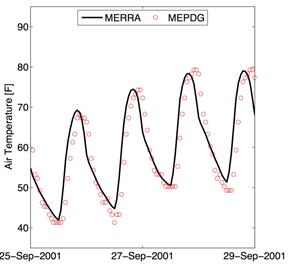
Figure 67. Graph. Typical comparison of diurnal temperature variations for MERRA versus MEPDG (QCLCD) data.
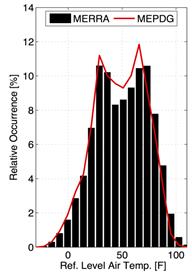
Figure 68. Graph. Typical comparison of hourly temperature frequency distributions for MERRA versus MEPDG (QCLCD) data.
The differences between QCLCD versus USCRN and MERRA versus USCRN hourly temperatures at coincident time points at a given location were used to compute bias and root mean squared error (RMSE). Figure 69 shows a typical frequency distribution for bias in the hourly temperatures for a single site located outside Chattanooga, TN. At this site, the MERRA data (average bias = 0.62 °F) compared better with the USCRN reference than did the QCLCD data (average bias = 2.00 °F), although the spread in the MERRA bias distribution was somewhat larger. At other sites, the QCLCD data compared better with the USCRN reference than did the MERRA data, but in most cases the average bias values were small—on the order of approximately 2 °F. Figure 70 is an example of a “worst-case” scenario for a site near Jacksonville, FL. Here the MERRA data (average bias = 5.52 °F) compared less well with the USCRN reference than did the QCLCD data. This is not surprising for a location right on the coast where half of the MERRA grid cell may be over land and half over water.
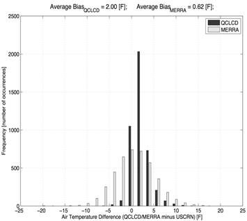
Figure 69. Graph. Frequency distribution of bias for QCLCD versus USCRN and MERRA versus USCRN hourly temperature values for a single site (outside Chattanooga, TN)—typical results.
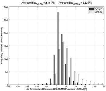
Figure 70. Graph. Frequency distribution of bias for QCLCD versus USCRN and MERRA versus USCRN hourly temperature values for a single site (near Jacksonville, FL)—worst-case results.
The calculations behind figure 69 and figure 70 were repeated at each of the other 273 collocated data sets to determine the average bias and RMSE in the QCLCD versus USCRN and MERRA versus USCRN hourly temperature values at each site. The distributions of the average bias and RMSE values are illustrated in figure 71 and figure 72, respectively. The average of the average bias across all 275 data sets was 1.14 °F for QCLCD versus USCRN and 2.53 °F for the MERRA versus USCRN comparisons. The spread of the MERRA bias distribution is slightly broader than for the QCLCD data. The average RMSE values (figure 72) were 3.68 °F for the QCLCD versus USCRN and 5.91 °F for the MERRA versus USCRN comparisons. Overall, both the QCLCD and MERRA data were different and warmer than the USCRN reference values, with the MERRA data being slightly warmer and more variable.
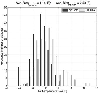
Figure 71. Graph. Frequency distribution of average hourly temperature bias across all sites for QCLCD versus USCRN and MERRA versus USCRN climate data.
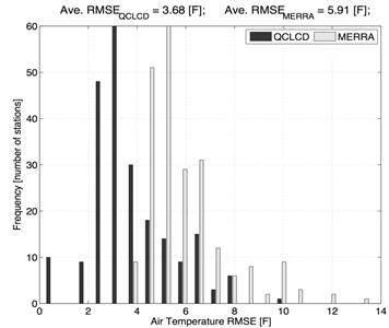
Figure 72. Graph. Frequency distribution of RMSE of QCLCD versus USCRN and MERRA versus USCRN hourly temperature values across all sites.
Precipitation at the Ground Surface
Analyses similar to those behind figure 71 and figure 72 were conducted for hourly precipitation rates for collocated USCRN, QCLCD, and MERRA stations. Only non-zero precipitation events were considered to better evaluate storm effects. More specifically, if at least one climate data source contained a non-zero hourly precipitation value, then that hour was included in the evaluation. If all of the data sources registered zero precipitation for an hour, then that hour was excluded. As shown in figure 73 and figure 74, both the QCLCD and MERRA data closely agree with USCRN precipitation measurements, but MERRA has 50 percent less average bias than does QCLCD (‑0.00059 inches/h versus -0.00106 inches/h). Further, data from numerous QCLCD stations contain significant negative bias relative to USCRN, which is consistent with rain gauge “under catch,” which is a known and pervasive problem with point-scale rain gauges.(68) The RMSE is also slightly lower in the MERRA estimates (0.032inches/h versus 0.036 inches/h for QCLCD).
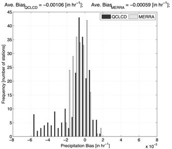
Figure 73. Graph. Frequency distribution of average hourly precipitation bias across all sites for QCLCD versus USCRN and MERRA versus USCRN climate data.
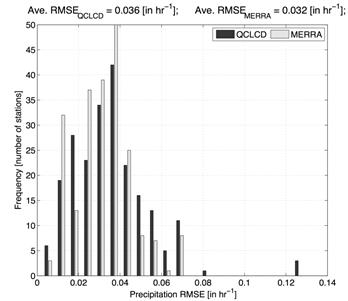
Figure 74. Graph. Frequency distribution of RMSE of QCLCD versus USCRN and MERRA versus USCRN hourly precipitation rates across all sites.
Comparisons of USCRN, COOP, and MERRA Daily Temperatures
The statistical analysis approach employed for hourly temperature data was repeated for daily mean, minimum, and maximum temperatures. The daily USCRN measurements were compared against daily values from the NWS COOP data as well as daily values derived from the original hourly MERRA estimates. Figure 75 shows the distribution of the collocated USCRN, COOP, and MERRA sites. The daily mean, minimum, and maximum temperatures from USCRN and MERRA were extracted from the original hourly temperature data. There was insufficient temporal overlap of the data for some of the sets of collated sites to enable computation of meaningful statistics. Statistical comparisons were made only where a large (> 100) number of daily readings were available for comparison.
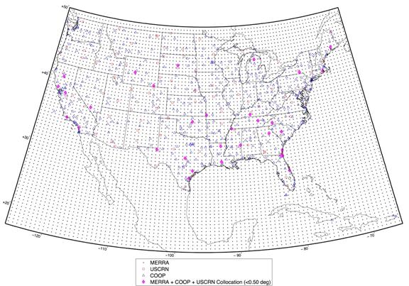
Figure 75. Map. Collocated USCRN, COOP, and MERRA data sets.
The average bias and RMSE for the COOP versus USCRN and MERRA versus USCRN daily mean temperature values were computed for each set of collocated sites. The distributions of these bias and RMSE values are illustrated in figure 76 and figure 77, respectively. The average of the average bias across all sites (figure 76) was 1.85 °F for COOP versus USCRN and 2.73 °F for the MERRA versus USCRN comparisons. The average RMSE values (figure 77) were 3.03°F for the COOP versus USCRN and 4.20 °F for the MERRA versus USCRN comparisons. Overall, both the COOP and MERRA daily mean temperatures were different and warmer than the USCRN reference values, with the MERRA data being slightly warmer and more variable.
Figure 78 and figure 79 summarize the average bias and RMSE for the COOP versus USCRN and MERRA versus USCRN daily minimum temperature values. The average of the average bias across all sites (figure 78) was 0.68 °F for COOP versus USCRN and 3.61 °F for the MERRA versus USCRN comparisons. The average RMSE values (figure 79) were 3.34 °F for the COOP versus USCRN and 6.04 °F for the MERRA versus USCRN comparisons. These findings suggest COOP does a better job of capturing the lower range of the diurnal air temperature than does MERRA. This is likely due to the spatial mismatch between the point-scale observations (i.e., USCRN and COOP) and grid cell scale estimates produced by MERRA. The adiabatic air temperature correction for elevation differential may also contribute to these differences.
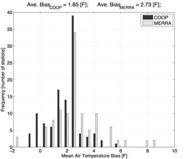
Figure 76. Graph. Frequency distribution of daily mean temperature bias across all sites for COOP versus USCRN and MERRA versus USCRN climate data.
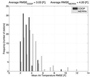
Figure 77. Graph. Frequency distribution of RMSE of COOP versus USCRN and MERRA versus USCRN daily mean temperature values across all sites.
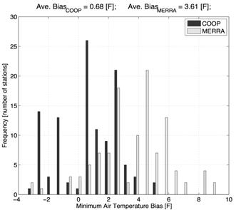
Figure 78. Graph. Frequency distribution of daily minimum temperature bias across all sites for COOP versus USCRN and MERRA versus USCRN climate data.
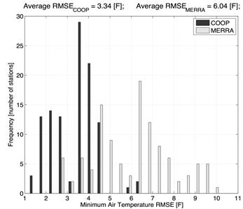
Figure 79. Graph. Frequency distribution of RMSE of COOP versus USCRN and MERRA versus USCRN daily minimum temperature values across all sites.
Figure 80 and figure 81 summarize the average bias and RMSE for the COOP versus USCRN and MERRA versus USCRN daily maximum temperature values. The average of the average bias across all sites (figure 80) was 2.46 °F for COOP versus USCRN and 2.88 °F for the MERRA versus USCRN comparisons. The average RMSE values (figure 81) were 3.46 °F for the COOP versus USCRN and 5.21 °F for the MERRA versus USCRN comparisons. Overall, both the COOP and MERRA daily maximum temperatures were different and warmer than the USCRN reference values, with the MERRA data being slightly warmer and more variable.
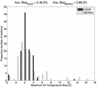
Figure 80. Graph. Frequency distribution of daily maximum temperature bias across all sites for COOP versus USCRN and MERRA versus USCRN climate data.
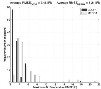
Figure 81. Graph. Frequency distribution of RMSE of COOP versus USCRN and MERRA versus USCRN daily maximum temperature values across all sites.
Comparisons of Hourly SIRS, QCLCD, and MERRA SSR
Although SSR is not a direct input in the MEPDG, it is the principal driver for pavement heating and cooling. Both USCRN and the SIRS were used as ground truth to evaluate the SSR issues.
The USCRN and SIRS stations use radiometers to directly measure the SSR at the site. The QCLCD sites (and, by association, the MEPDG weather station data) do not have radiometers and thus do not measure SSR. In the EICM calculations embedded in the MEPDG software, the downwelling shortwave radiation is determined using an empirical equation that is a function of cloud cover as shown in figure 82:

Figure 82. Equation. Downwelling shortwave radiation.
Where Qs downwelling (incoming) shortwave radiation, asis the surface shortwave absorptivity of the pavement, and R is the shortwave radiation at the top of the atmosphere that is a function of latitude and seasonally varying solar declination. The term Sc is the percentage of sunshine computed as Sc=1-NW, where N is a cloud base factor equal to 0.9 to 0.8 for cloud heights of 1,000 to 6,000 ft, and W is the average cloud cover during day or night.(66) The constants A and B are empirical terms that account for diffuse scattering and adsorption by the atmosphere; the values of A and B incorporated in the MEDPG, which are based on data for the upper Midwest and Alaska, equal 0.202 and 0.539, respectively.(58) This empirical expression is required only with the QCLCD measurements because USCRN, SIRS, and MERRA all provide direct measurement or estimates of downwelling shortwave radiation.
Figure 83 and figure 84 summarize the average bias RMSE for the QCLCD versus USCRN and MERRA versus USCRN SSR values across all collocated data sets. Recall that each point in figure 83 represents the average of the hourly SSR bias values over the entire duration of temporally matched data series at a single site. Each point in figure 84 represents the RMSE of the hourly SSR values at a single site. The average of the average bias across all sites (figure 83) was 20 W/m2 for QCLCD versus USCRN and 51 W/m2 for the MERRA versus USCRN comparisons. For perspective, these values can be compared against the maximum shortwave radiation at the top of atmosphere equal to 1,366 W/m2; the bias values are less than 4 percent of this maximum. The average RMSE values (figure 84) were 176 W/m2 for the QCLCD versus USCRN and 166 W/m2 for the MERRA versus USCRN comparisons. Overall, both the QCLCD and MERRA SSR values were different and slightly higher than the USCRN reference values.
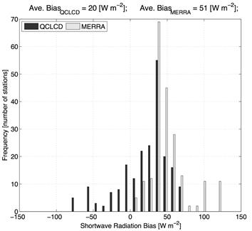
Figure 83. Graph. Frequency distribution of SSR bias across all sites for QCLCD versus USCRN and MERRA versus USCRN climate data.
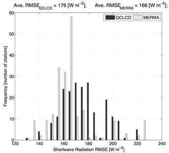
Figure 84. Graph. Frequency distribution of RMSE of QCLCD versus USCRN and MERRA versus USCRN SSR values across all sites.
Five SIRS sites were used for a more in-depth evaluation of SSR differences. The SIRS sites, which are all located in the southern Great Plains, were designed specifically for collecting SSR data using very sophisticated and accurate radiometers. Figure 85 and figure 86 summarize the bias and RMSE for QCLCD versus SIRS and MERRA versus SIRS climate data as a function of cloud cover. Several important insights can be drawn from these figures. During periods of low cloud cover—i.e., periods of maximum SSR and pavement heating—the QCLCD has high positive biases and variability relative to MERRA. MERRA has a greater positive bias during periods of heavy cloud cover but these conditions generally do not correspond to the extremes for pavement performance.
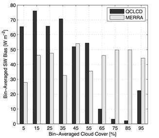
Figure 85. Graph. SSR bias as a function of cloud cover for QCLCD versus SIRS and MERRA versus SIRS climate data.
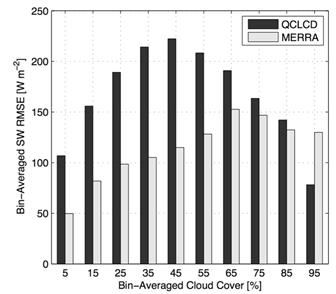
Figure 86. Graph. SSR RMSE as a function of cloud cover for QCLCD versus SIRS and MERRA versus SIRS climate data.
A complementary trend can be observed as a function of season. Figure 87 shows the bias in daily averaged SSR for QCLCD versus SIRS and MERRA versus SIRS for each month during the analysis period. The QCLCD data show much higher biases than MERRA during the summer months of May through September—the critical period of maximum pavement heating. Conversely, the MERRA data show higher biases during the later winter and spring months of January through April; these are generally less critical periods for pavement heating and performance. The RMSE values for both sets of climate data are relatively similar (figure 88).
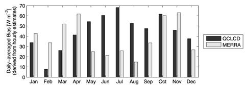
Figure 87. Graph. SSR bias as a function of season for QCLCD versus SIRS and MERRA versus SIRS climate data.
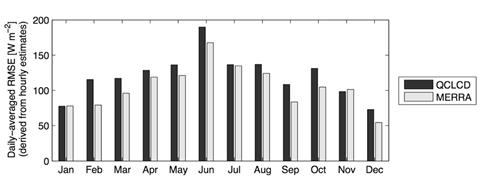
Figure 88. Graph. SSR RMSE as a function of season for QCLCD versus SIRS and MERRA versus SIRS climate data.
The overall conclusions drawn from these data are as follows. The SSR values from the QCLCD data estimated empirically using the equation in figure 82 and the values predicted by the MERRA approach show similar bias on an annual basis. However, when disaggregated into bias as a function of cloud cover and bias as a function of month of year, the QCLCD data tend to have higher positive biases during the critical extreme-temperature periods for the pavement—low cloud cover and summer months—compared with the MERRA data. This may be a consequence of the empirical relation used in the EICM to estimate SSR based on top-of-atmosphere radiation and cloud cover. Use of the MERRA direct SSR data eliminates the need for this type of empirical relationship.
Conclusions From Statistical Comparisons
The overall conclusions from the statistical comparisons of the various climate data sources can be summarized as follows:
Table 13. Summary of statistical comparisons of QCLCD versus USCRN and MERRA versus USCRN hourly climate data.
Bias | RMSE | |||
QCLCD |
MERRA |
QCLCD |
MERRA | |
| Average Hourly Temperature (°F) | 1.14 |
2.53 |
3.68 |
5.91 |
Table 14. Summary of statistical comparisons of COOP versus USCRN and MERRA versus USCRN daily climate data.
| Bias | RMSE | |||
COOP |
MERRA |
COOP |
MERRA | |
| Average Daily Mean Temp (°F) | 1.85 |
2.73 |
3.03 |
4.20 |
| Average Daily Min Temp (°F) | 0.68 |
3.61 |
3.34 |
6.04 |
| Average Daily Max Temp (°F) | 2.46 |
2.88 |
3.46 |
5.21 |
COMPARISONS OF PREDICTED PAVEMENT PERFORMANCE
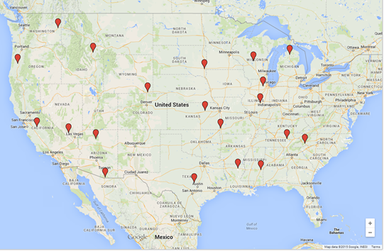
Pavement performance as predicted by the MEDPG models incorporated in the Pavement ME Design® software was evaluated using the MEPDG weather data files provided with the software (derived from the QCLCD and ULCD products from NCDC) and the MERRA climate data for collocated sites and congruent time series. A total of 20 sites were analyzed; their distribution across the contiguous United States is shown in figure 89.
It would have been ideal to evaluate MEPDG performance predictions using the USCRN ground truth data in addition to the MEDPG and MERRA weather time series. However, the USCRN data do not include the wind speed and cloud cover data required for the MEPDG models. Several attempts were made to synthesize these missing data from other sources but none was satisfactory.
Both new flexible pavements and new JPCP were analyzed. The pavement structures, traffic loads, material properties, and other inputs for the analysis correspond to the medium traffic cases for the sensitivity analyses described in Schwartz et al.(1) All analyses were performed using version 2.0 of the Pavement ME Design® software.
©2014 Google®
Figure 89. Map. Sites used for evaluation of MEPDG performance predictions using MEPDG and MERRA climate data.(69)
Comparisons of flexible pavement performance as predicted by the MEPDG using MERRA versus MEPDG weather data are shown in figure 90 for total rutting, figure 91 for AC rutting, figure 92 figure 92 for alligator fatigue cracking, figure 94 for top-down fatigue cracking, and figure 95 for roughness. In all cases, the predictions are clustered tightly although not perfectly along the respective lines of equality. This is consistent with the close but not perfect agreement found among these climate data time series in the statistical comparisons described previously. The worst agreement in performance predictions is for top-down fatigue cracking (figure 94). However, this model is also generally viewed as unreasonably sensitive and unrealistic; a replacement for the current top-down fatigue cracking model is currently being developed in NCHRP Project 1-52.
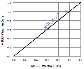
Figure 90. Graph. Comparison of MEPDG total rutting predictions (inches) using MERRA versus MEPDG weather data.
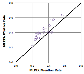
Figure 91. Graph. Comparison of MEPDG AC rutting predictions (inches) using MERRA versus MEPDG weather data.
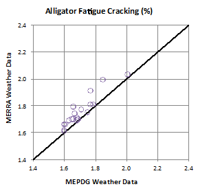
Figure 92. Graph. Comparison of MEPDG alligator fatigue cracking predictions using MERRA versus MEPDG weather data.
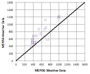
Figure 93. Graph. Comparison of MEPDG top-down fatigue cracking predictions (ft/mi) using MERRA versus MEPDG weather data.
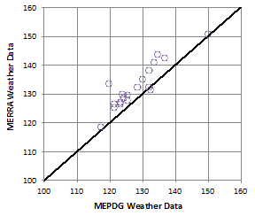
Figure 94. Graph. Comparison of MEPDG flexible pavement IRI predictions (inches/mi) using MERRA versus MEPDG weather data.
Comparisons of rigid JPCP pavement performance as predicted by the MEPDG using MERRA versus MEPDG weather data are shown in figure 95 for transverse cracking, figure 96 for joint faulting, and figure 97 for roughness. In all cases, the predictions are clustered tightly although not perfectly along the respective lines of equality. This is consistent with the close but not perfect agreement found among these climate data time series in the statistical comparisons described previously. The agreement between the MERRA versus MEPDG weather data cases for rigid pavement performance is somewhat less than for flexible pavements. However, this is consistent with the fact that rigid pavement performance is more sensitive to shorter term (e.g., diurnal) temperature variations and thus to the differences between MERRA versus MEPDG weather data over short time periods.
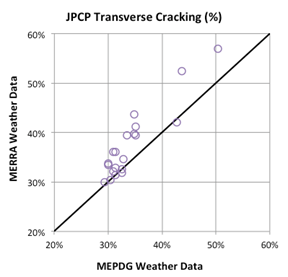
Figure 95. Graph. Comparison of MEPDG JPCP transverse cracking predictions using MERRA versus MEPDG weather data.
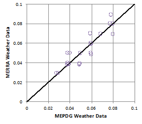
Figure 96. Graph. Comparison of MEPDG JPCP joint faulting predictions (inches) using MERRA versus MEPDG weather data.
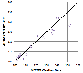
Figure 97. Graph. Comparison of MEPDG rigid pavement IRI predictions (inches/mi) using MERRA versus MEPDG weather data.
Overall, the comparisons of MEPDG predicted performance for both flexible and rigid pavements using MERRA versus MEPDG weather data are close and acceptable for engineering design. Based on the earlier statistical comparisons among the various climate data sources, the agreement in predicted performance using MERRA versus USCRN ground truth and/or MEPDG versus USCRN would likely show similar scatter in agreement as seen in figure 90 through figure 97. However, it is impossible to demonstrate this because the USCRN data lack the wind speed and cloud cover inputs required by the MEPDG software.
The results of the more extensive statistical and pavement performance comparisons reported here support the original recommendation that LTPP should adopt MERRA as a data source for its next update to the climate data module and develop a tool to extract and use this data for engineering applications.