U.S. Department of Transportation
Federal Highway Administration
1200 New Jersey Avenue, SE
Washington, DC 20590
202-366-4000
Federal Highway Administration Research and Technology
Coordinating, Developing, and Delivering Highway Transportation Innovations
| REPORT |
| This report is an archived publication and may contain dated technical, contact, and link information |
|
| Publication Number: FHWA-HRT-14-020 Date: January 2015 |
Publication Number: FHWA-HRT-14-020 Date: January 2015 |
Because a current observational before-after traffic safety evaluation is being performed for the HFST under another FHWA contract (Evaluation of Low-Cost Safety Improvements Pooled Fund Study), this study did not assess crash frequency or severity. Rather, the current study assesses the speed effects of HFST, as well as encroachments onto the shoulder or into the opposing travel lanes.
This section describes the HFST site selection criteria, site characteristics and data-collection, and analysis methods used for evaluation.
HFST can improve the skid-resistance properties of highway pavements. These surfaces are typically cold-applied treatments using a resin to bond polish- and abrasion-resistant aggregate to an existing pavement structure.(68) HFST has been applied in the United States on horizontal curves along roadway segments and on freeway interchange ramps; to delineate pedestrian, bicycle, and bus lanes; and on bridge decks. The roadway segment treatments are intended to reduce roadway departure crashes on horizontal curves and are applicable to the present study.
Through outreach efforts to State transportation agencies, the research team identified several HFST horizontal curve treatment sites on two-lane rural roadways in West Virginia for use in this study. The West Virginia Department of Transportation (WVDOT) identified many high- risk locations on horizontal curves that were subject to run-off-road crashes and, in an effort to reduce injuries and fatalities, began implementing HFST in May 2011 as a low-cost, site-specific safety solution on the identified high-risk locations. The following roadways were selected for use in this study:
In addition to the four treatment sites, the research team identified three corresponding control sites. One of these control sites was located on the same route as two treatment sites and thus served as a control site for both treatment locations.
Table 6 shows the various site-specific data for all of the treatment and control sites. The research team selected treatment and control sites with the intent of collecting data at locations with varying horizontal curve radii. Control sites were located along the same route as the treatment sites. The research team tried to find control sites that were similar to the treatment sites with respect to horizontal curve direction, curve radius, curve length, superelevation, and PSL (including the advisory speed). The evaluation results section of this chapter provides a plan view sketch and details concerning each data-collection site, which show the data-collection locations with respect to the limits of each curve.
Table 6. West Virginia HFST site characteristics.
Site Number |
County |
Route |
Radius of Curve (ft) |
Length of Curve (ft) |
Curve Direction |
Vertical Grade (percent) |
Superelevation (percent) |
Posted/ Advisory Speed Limit (mph) |
T1 |
Randolph |
WV 32 |
680.4 |
1,080.5 |
Right |
-0.5 |
8.0 |
55/40 |
C1 |
Randolph |
WV 32 |
1073.3 |
1,213.6 |
Right |
-3.5 |
7.0 |
55/50 |
T2 |
Pendleton |
U.S. 33 |
210.0 |
539.2 |
Left |
-8.0 |
6.0 |
55/25 |
C2 |
Pendleton |
U.S. 33 |
264.8 |
693.6 |
Left |
-7.5 |
8.5 |
55/25 |
T3 |
Randolph |
U.S. 219 MM 6.32 |
605.1 |
753.8 |
Right |
-2.0 |
11.0 |
55/30 |
C3/C4 |
Randolph |
U.S. 219 |
544.6 |
826.9 |
Right |
-6.5 |
12.0 |
55/30 |
T4 |
Randolph |
U.S. 219 MM 5.81 |
272.9 |
673.4 |
Right |
-3.0 |
12.0 |
55/25 |
MM = Mile Marker
The Before-Period Data Summary section later in this chapter describes the specific characteristics of each data-collection site.
Contractors for WVDOT installed HFST at the test sites between May 22, 2012, and June 4, 2012. HFST was applied by a self-contained, fully automated application vehicle in one pass up to 12 ft wide.
OPERATING SPEED EVALUATION METHODOLOGY
The research team employed observational before-after study to evaluate the effects of HFST on vehicle operating speeds. Because the intent is that HFST increases the available friction at the road surface–tire interface, this treatment may increase vehicle operating speeds. The basis for this hypothesis is that HFST improves the friction supply, and therefore, drivers may increase their travel speed and demand higher friction. Further, the HFST provides a color contrast when applied adjacent to older pavement surfaces and appears similar to a new pavement surface. This appearance may also encourage higher vehicle operating speeds. However, because an HFST typically is applied only between the limits of the horizontal curve (point of curvature (PC) to point of tangent (PT)), it is also possible that this treatment will have little influence on driver speed choice. An increase or no change in operating speeds will not necessarily imply a treatment failure. Comparisons of required versus available side friction for the speeds observed during this study, combined with the results of an ongoing FHWA safety evaluation of HFST, will indicate treatment effectiveness. The research team has also included an encroachment evaluation to supplement the speed evaluations and the parallel safety effort. Figure 16 and figure 17 show an example of a curve without the high-friction surface and the same curve with the high-friction surface, respectively.
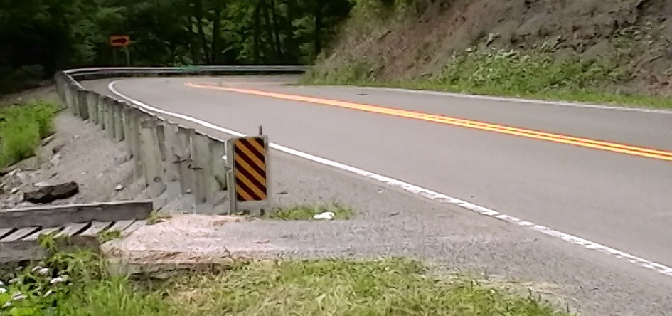
Source: Pennsylvania State University
Figure 16. Photo. Photograph of a horizontal curve without the HFST.
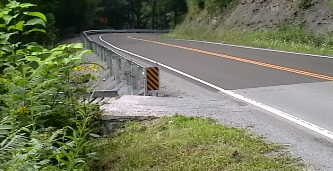
Source: Pennsylvania State University
Figure 17. Photo. Photograph of a horizontal curve with the HFST.
The observational before-after evaluations were performed at four treatment sites, and three corresponding control sites. (One control site was located on the same route as two treatment sites and thus served as a control site for both treatment locations.) The control sites were located on the same roadway and had similar geometric features (i.e., lane width and curve radius) when compared with the treatment sites. The team collected data at each site for one before period and two after periods. This section of the report describes the data-collection equipment and locations, sample size requirements, data-collection periods and durations, and the statistical analysis methodology for the speed study.
Data-Collection Equipment and Locations
The research team used on-pavement traffic sensors to collect speed data. HI-STAR® sensors use vehicle magnetic-imaging technology to record vehicle count, speed, headway, time, pavement temperature, pavement condition (dry or wet), and vehicle length. These sensors are nonintrusive, thus reducing the possibility of drivers adjusting their speeds because of visible equipment and human observers. The dimensions of the sensors are 6.5 by 5.5 inches with a thickness of 0.625 inches. Each sensor is placed in the center of the travel lane and as a vehicle passes over it, the sensor captures changes in the magnetic field. A rubber cover protected the sensor and reduced its conspicuity on asphalt surfaces. The research team used Highway Data Management (HDM) software to program the sensors prior to field data collection—the internal clock was set to record vehicle speeds for up to 12 to 16 h, including both daytime and nighttime periods, depending on the time of day and traffic volumes present at the study locations. The research team also used HDM software to download the data from the sensors into Microsoft® Excel spreadsheets.
The research team placed the sensors at three different points at each study site to collect speed data at the treatment and comparison sites: 1) approximately 300 ft prior before the beginning of the horizontal curve,1 2) at the beginning of the horizontal curve (PC), and 3) at the midpoint of the horizontal curve. Figure 18 shows the data-collection locations along a study site. HI- STAR® sensors are capable of adding time stamp information to each vehicle collected at a particular location so vehicles can be tracked. A sensor was also placed in the opposing travel lane, near the midpoint of the horizontal curve, to determine whether a vehicle was present at the same time that a vehicle was present in the analysis direction.
The traffic volumes at the study locations were low, with daily traffic volumes ranging from approximately 700 to 1,600 vehicles per day. The probability of an opposing vehicle near to or on the horizontal curve at the same time as the subject vehicle was small. However, the analysis described below did consider the presence of a vehicle in the opposing travel lane.
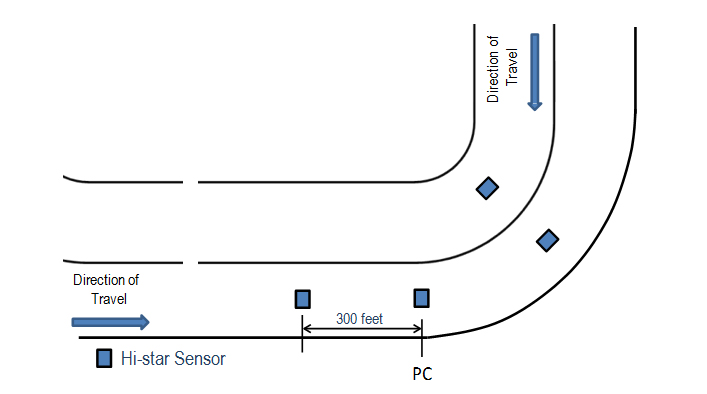
Figure 18. Diagram. Location of traffic sensors for treatment and control sites (not to scale).
The research team used the equation shown in figure 19 to determine the sample size when estimating the mean speed from a population of speeds, while minimizing the tolerable error in field measurements.(69)

Figure 19. Equation. Minimum number of measured speeds.
Where:
N = minimum number of measured speeds.
S = estimated sample standard deviation (SD), mph.
K = constant corresponding to the desired confidence level.
E = permitted error in the average speed estimate, mph.
To obtain a range of possible sample sizes, multiple values for the confidence level K were considered. The values correspond to confidence levels of 90, 95, and 99 percent. The permitted error in the average speed estimate E has been included as a conservative value of ±1 mph. The estimate of sample SD S is a function of area type and highway type. The input value of 5.3 is representative of a rural, two-lane highway.(69) Table 7 summarizes the resulting sample size estimates for the proposed confidence interval, permitted error, and SD estimates.
Table 7. Sample size determination.
Confidence Level (percent) |
K |
N |
90 |
1.64 |
76 |
95 |
1.96 |
108 |
99 |
2.58 |
187 |
As table 7 shows, the estimated sample size for the 95th percentile confidence level is approximately 110 free-flow passenger car speeds. It should be noted that collecting the minimum sample size depends on the traffic characteristics at each study site. The research team attempted to collect the minimum sample size during both daytime and nighttime periods, which covered one 12- to 16-h period per site (6−8 h of daytime and 6−8 h at night).
When comparing the difference in means for two different data-collection periods, the expected effect size (i.e., difference in mean speeds) is an important consideration. In this case, the equation shown in figure 20 was used to estimate the sample size in an observational before-after study:
Figure 20. Equation. Sum of the sample in before-after comparison groups.
Where:
N = sum of the sample in both comparison groups (before-after).
s = SD of the comparison groups (assumed equal) (mph).
zcritical = level of statistical significance assumed from the standard normal distribution.
zpower = desired statistical power from the standard normal distribution.
D = minimum expected difference between the sample means (mph).
Table 8 shows different sample size estimates, assuming that the SD in speed is 5.3 mph for varying levels of critical and power statistics and for different minimum expected differences in sample means.
Table 8. Sample size estimates for comparative research studies.
|
Difference in Means (mph)
|
Level of Statistical Significance (Zcritical)
|
|||
|
90 percent (zcritical = 1.645)
|
95 percent (zcritical = 1.96)
|
|||
|
Deisred Statistical Power (zpower)
|
Deisred Statistical Power (zpower)
|
|||
|
90 percent (zpower = 1.282) |
95 percent (zpower = 1.645) |
90 percent (zpower = 1.282) |
95 percent zpower = 1.645) |
|
| 1.0 |
500 |
822 |
709 |
1,169 |
2.0 |
125 |
206 |
177 |
292 |
3.0 |
56 |
91 |
79 |
130 |
4.0 |
31 |
51 |
44 |
73 |
5.0 |
20 |
33 |
28 |
47 |
Because the treatments in the current study are original and little information exists to determine the expected difference in means between the before and after periods, the research team used 2.0 mph as a practical difference. In this case, 95-percent statistical significance and power required a minimum sample size of 292 free-flow passenger cars to be included in the combined before and after samples (i.e., 146 free-flow speeds per data-collection period). The 110 free- flow passenger car speeds recommended for each data-collection period based on the equation in Figure 19 would yield 95-percent statistical significance and more than 90-percent statistical power, if a 2.0 mph difference in means was computed between the before and after samples. As a result, the research team sought to measure at least 110 free-flow vehicle speeds during each 12- to 16-h collection period; however, if additional free-flow vehicles were available for analysis, the entire sample was used to compare the before with after mean speeds.
Data-Collection Periods and Durations
Speed data were collected on weekdays only and during both daytime and nighttime periods. Only free-flow vehicles were included in the evaluation sample. The definition of a free-flow vehicle also meant no opposing vehicles were present that could influence the subject vehicle. The extent to which observations with opposing vehicles could be screened depended on the sample size and the estimated effect of the opposing vehicles as described above. Based on previous studies, free-flow vehicles were identified as those vehicles traveling with a minimum headway of 5 s. (70,71) Data were collected at each study site during favorable driving conditions—clear weather with normal visibility (no fog) and dry roadway conditions, without the presence of standing water from an earlier rain. These requirements increased the likelihood that drivers were selecting their operating speeds based solely on the physical roadway and roadside features at each site; during and after HFST implementation, any changes in operating speeds could then be associated with the HFST treatment. The data-collection session was long enough so that sufficient data were collected to satisfy the sample size requirements after the data were screened (i.e., after non-free-flow passenger cars were eliminated from the database).
The study methodology was an observational before-after study. The before data were collected before implementing the HFST on horizontal curves. All before data collection occurred during summer 2012. Two after data collection periods were included in the evaluation. The first after period occurred approximately 1 month after implementing the HFST to minimize the novelty effects associated with the treatment—these data were also collected during summer 2012. A second after period occurred approximately 1 year after implementing the HFST, during summer 2013. The research team chose a 1-year interval between the after periods to minimize seasonal effects and to assess long-term novelty effects of the treatment. It was anticipated that the skid- resistant qualities of the HFST would decrease after 1 year because of vehicle tire abrasion and likely winter maintenance on roadways in West Virginia.
Before beginning the data analysis, all raw data from the treatment and control sites were screened to exclude all vehicles that were not passenger cars and that were not considered free- flow vehicles, as described previously. It was anticipated that vehicles present in the opposing travel lane would influence the speed of free-flow vehicles in the subject travel lane; therefore, the research team added an indicator variable to the data files to identify free-flow vehicles in the subject travel lane that were measured in the presence of an opposing vehicle. The research team excluded missing data values from the analysis. The research team carefully evaluated data points considered outliers to determine whether to exclude them in the analysis. Examples of outliers include vehicles traveling at very low speeds or entering or exiting at nearby driveways.
The research team calculated after data screening and mean operating speeds at each sensor location for all treatment and control sites and all data-collection periods. The team then compared corresponding speed parameters at each site for each data-collection period by calculating the numerical differences in these speed parameters. The team applied the t-statistic for independent samples to determine whether the differences in mean speed were statistically significant. Statistically significant changes in mean operating speeds indicated that the observed speeds were different in the two time periods compared. The t-statistic is commonly used to test the hypothesis of differences in population parameters.(72) In this study, the null and alternative hypotheses for testing the differences in two population mean speed measures, μ1 and μ2, were the following:
At each study site, a t-statistic is calculated for each sensor location and between data-collection periods. Independent two-sample t-statistics is applied to test for the difference between two sample means at each study site. The t-statistic for large samples with known variables is calculated using the equation shown in figure 21: (73)
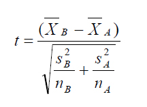
Figure 21. Equation. t-statistic to test for the difference between two sample means at each study site.
Where:
![]() B ,
B , ![]() A = mean speed for the before and after periods.
A = mean speed for the before and after periods.
sB, sA= SD of speed for the before and after periods.
nB, nA= sample size in before and after periods.
In figure 21, both the first and second after periods were compared with the before period and to each other, using data from the treatment and comparison sites.
The degrees of freedom (df) for the independent samples t-statistic is nA + nB - 2. The critical value when α = 0.05 for a one-tail test is 1.645. The null hypothesis is rejected when the computed t-test exceeds the critical value, thus concluding that the mean speeds being compared differ between the two collection periods being considered. An alternative method to determine the statistical significance of HFST on mean speed is the p-value associated with the t-statistic. A low p-value (i.e., less than or equal to 0.05) indicates a high probability that implementing the
HFST influenced mean speeds between two data-collection periods. The team computed t-statistic and p-value for each pair of collection periods at each study site. It was anticipated that the difference in mean speeds at the control sites would not be statistically significant. However, if there is a statistically significant difference in mean speeds between any of the data-collection periods, the magnitude of this difference would need to be taken into account. In this case, the research team added or subtracted, depending on whether the difference is positive or negative, to the numerator in figure 21. As such, the mean speed difference computed at the treatment sites was adjusted to account for statistically significant mean speed differences at the treatment sites.
The research team also used the t-test for independent samples to compare the before and after mean difference in vehicle speeds between the PC and the curve midpoint. The comparison of mean delta v, where delta v is the curve PC speed minus the curve midpoint speed, was made in the same way as the mean speed comparisons.
In addition to the t-test, the percentage of vehicles exceeding the PSL and the advisory speed at the treatment and control sites was calculated and compared between data-collection periods. The percentage of speeding vehicles, PS, was computed using the equation shown in figure 22.
Figure 22. Equation. Percentage of speeding vehicles.
Where:
x = number of vehicles exceeding the PSL.
n = the total number of vehicles in the sample.
By comparing the number of vehicles exceeding the PSL in two data-collection periods, it can be determined whether the HFST is associated with reducing the proportion of PSL violations. The percent reduction in speeding vehicles %RS from period 1 to period 2, at the treatment and control locations, is computed using the equation shown in figure 23.
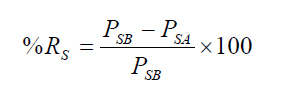
Figure 23. Equation. Percent reduction of speeding vehicles.
Where:
PSB= the proportion of vehicles speeding during the before data-collection period.
PSA= the proportion of vehicles speeding during the after data-collection period. (Note that there will be two after periods for each location.)
To determine whether the proportion of vehicles exceeding the PSL at the treatment and control locations changed between data-collection periods, a Z-test for independent samples was computed. The null and alternative hypotheses for the test are the following:
The Z-statistic used to determine the statistical difference between the two proportions is computed using the equation shown in figure 24.(73)
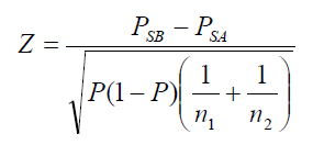
Figure 24. Equation. Z-statistic to determine the speed difference between a pair of before and after periods.
Where PSB and PSA are the sample proportions from figure 23, n1 and n2 are sample sizes for the corresponding proportions being considered, and P is the combined proportion in both samples, computed using the equation shown in figure 25.

Figure 25. Equation. Combined proportion of vehicles speeding during the before and after data-collection periods.
Similar to the t-statistic, the Z-statistic is associated with a p-value. A p-value of 0.05 or less rejects the null hypothesis and concludes that the HFST is effective in reducing the number of vehicles exceeding the speed limit at the 95-percent confidence level.
The final speed performance metric considered in the present study is speed variance. A two- sided F-test is used to compare the variances of vehicle operating speed in the before and after periods. The F-test is computed using the equation shown in figure 26.

Figure 26. Equation. F-test to compare the speed variance in the before and after periods.
This equation has an F-distribution with (nB – 1) numerator degrees of freedom and (nA– 1) denominator degrees of freedom. When the computed F-test exceeds the critical value, the null hypothesis is rejected, and the conclusion is that the speed variance differs between the before and after periods.
HFST ENCROACHMENT EVALUATION METHODOLOGY
The purpose of the encroachment evaluation was to determine whether the HFST changes the proportion of vehicles that cross either the edge line or centerline on two-lane rural highways in West Virginia. Because the HFST increases the coefficient of road adhesion, it was hypothesized that the proportion of lane-line encroachments would decrease. The following sections describe the encroachment evaluation data collection and analysis.
Data-Collection Locations and Periods
Data collection took place at the same locations described above in the speed evaluation section. To identify lane-line encroachments, the research team deployed digital video recorders at all treatment and comparison site locations. A single recorder was positioned on the approach tangent, near the PC location, to record vehicles traversing the first half of the horizontal curve (PC to midpoint). Video data were recorded during daylight hours only in the before period (2 to 4 h per collection period at each site), and during two after treatment periods. The first after period occurred within the first month after applying the HFST to a horizontal curve, and the second after period occurred approximately 1 year after installing the HFST treatment. Data collection at the comparison sites occurred on the same days as the treatment site data collection.
The research team collected the video data and reviewed it on a computer. The research team then tabulated the total number of vehicles observed and the number of vehicles that crossed the edge line and the centerline of the roadway within the limits of the PC and midpoint of the horizontal curve. The proportion of vehicles encroaching on the edge line or centerline was then computed using the equation shown in figure 27.

Figure 27. Equation Proportion of vehicles encroaching on the edge line or centerline.
Where:
Pe= proportion of vehicles encroaching on the edge line or centerline.
x = number of vehicles encroaching on the edge line or centerline.
n = number of vehicles observed during data-collection period.
To determine whether the proportion of vehicles encroaching on a lane line at the treatment and control locations changed between the before and after data-collection periods, the team computed a Z-test for independent samples. The null and alternative hypotheses for the test are the following:
The Z-statistic used to determine the statistical difference between the two proportions is shown in figure 28.
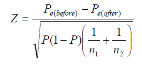
Figure 28. Equation. Z-statistic to determine the proportion of vehicles encroaching on a lane line during the before and after data-collection periods.
Where Pe(before ) and Pe(after) are the sample proportions from figure 23, n1 and n2 are sample sizes for the corresponding proportions being considered, and P is the combined proportion in both samples, computed using the equation in figure 29.

Figure 29. Equation. Combined proportion of vehicles encroaching on a lane line between the before and after data-collection periods.
Similar to the t-statistic, the Z-statistic is associated with a p-value. A p-value of 0.05 or less rejected the null hypothesis and concluded that the HFST is effective in reducing the number of vehicles exceeding the speed limit at the 95-percent confidence level.
FRICTION EVALUATION METHODOLOGY
The research team also measured roadway surface friction before and after implementing HFST. The following is a discussion of the friction testing methods.
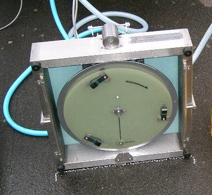
The research team used a dynamic friction (DF) tester to evaluate the skid resistance of the HFST and comparison site locations. All testing was performed in accordance with ASTM E1911-09a, Standard Test Method for Measuring Pavement Surface Frictional Properties Using the Dynamic Friction Tester. The DF tester measures the necessary torque to turn three small rubber pads in a circular path on the measured surface at different speeds. The apparatus consists of a horizontal spinning disk fitted with three spring-loaded rubber sliders that contact the paved surface as the disk rotational speed decreases because of the friction supplied between the sliders and the paved surface. A water supply unit delivers water to the paved surface being tested. The torque generated by the slider forces, measured during the spin down, is then used to calculate the friction supply as a function of speed. Typical test speeds range from 55 mph down to 3 mph. The device uses an electric motor to spin the measuring disc at the desired speed and an electromagnetic device to lower the spinning disk to the ground at the highest speed revolution.
The device is equipped with a rotational speed measurement device together with a rotational torque and a downward load measurement sensor. Figure 30 shows the DF tester.
Source: Pennsylvania State University
Figure 30. Photo. Dynamic friction tester.
The device is portable and was manually placed on the pavement surface where the test took place. The research team used a laptop computer to control the test and record the data. Once the test was initiated, the electronic motor first accelerated the disk to the standard spinning speed of 55 mph. The electromagnetic release mechanism then dropped the spinning disk to the ground, at which time automated data acquisition began. The test was completed when the disk came to a complete stop. The raw data were then filtered—the friction supply at the pavement-rubber disk interface was calculated from the measured and filtered torque and loading forces based on an internal algorithm within the testing apparatus.
The team used a circular texture (CT) meter along with the DF tester to measure road surface texture characteristics. The meter is designed to measure surface texture on the same circular track as the DF tester. The CT meter calculates and reports the mean profile depth (MPD) of the road surface and the International Friction Index (IFI).
The following describes the data-collection protocol with the number of measurements and the placement of measurements.
The research team used the DF tester and CT meter to measure all treatment and control sites included in the speed study. A single before period, and two after periods were included in the data-collection process. These periods corresponded with the time periods described previously for the speed and encroachment data collection. The research team used the following testing protocol:
The research team derived a representative friction supply curve for each test segment. The curves were plotted to illustrate the difference in friction supply before and after application of the HFST. Figure 31 shows a sample illustration of road friction curves produced using the measurement protocol described above. The research team used this analysis to determine the absolute change in friction supply at various locations approaching and along the horizontal curve at the treatment and control sites.
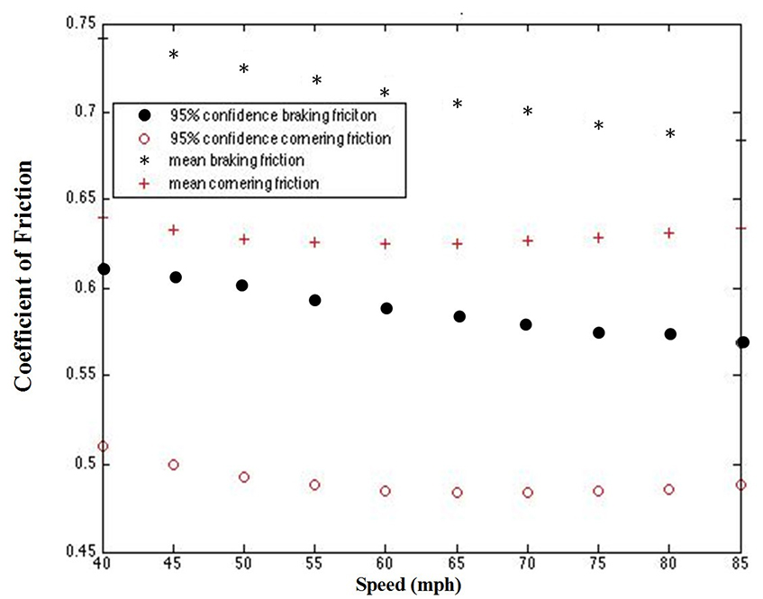
Figure 31. Graph. Road friction curves (for illustrative purposes only).
In addition to the friction curves, the research team used the speed data collected during the speed study to compute the difference in friction supply and the friction demanded by vehicles traversing horizontal curves at the treatment and control locations. The friction demand was computed using the point-mass model, using the equation shown in figure 32.

Figure 32. Equation. Side friction demand.
Where:
f = side friction demand.
V = vehicle operating speed (mph).
R = radius of horizontal curve (ft);
e = rate of superelevation (percent).
During the friction testing, the research team used a digital slope meter to measure the superelevation at the midpoint of each horizontal curve. The team then computed the descriptive statistics from the distributions of friction demand (e.g., mean, SD, 95th percentile) at each treatment and control curve location to the friction supply distribution. The margin of safety, based on the difference between the distributions of friction supply and demand, was computed for each treatment and control location.
Speed, friction, and encroachment data were collected before implementing the HFST application at seven sites near Elkins, WV. Data were collected at four treatment sites and three comparison sites. One comparison site was located between two treatment sites on U.S. Route 219, and was therefore used as a basis to compare the before and after operational performance at the two adjacent treatment sites. This section of the report describes the specific characteristics of each data-collection site, as well as the speed and other operational data-collection protocols employed at each site in the before period. This section of the report also provides results of the before analysis.
West Virginia Route 32 Treatment Site (T1 in Table 6)
The direction of travel for speed data collection was from south to north (bottom left to top right in figure 33). There was a cut slope on the inside of the curve, which limited horizontal sight distance along the curve. The radius of curve and the curve length, calculated using Google Earth™, were found to be 680.43 ft and 1,080 ft, respectively. The superelevation for this curve was 8.0 percent and the vertical grade was -0.5 percent, based on manual field measurements with a digital slope meter. The PSL was 55 mph. As figure 33 shows, there was a curve-to-the- right warning sign (W1-2) with a 40-mph advisory speed plaque (W13-1P). The travel lanes were 10 ft wide, and there was a 4-ft paved shoulder on both sides
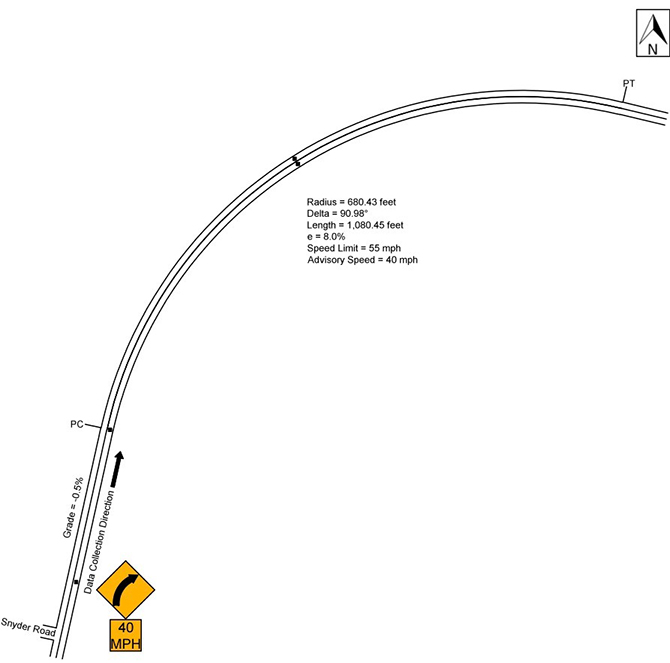
Figure 33. Diagram. Geometric layout of WV Route 32 treatment site (not to scale).
At this site, the research team collected data 300 ft before the PC, at the PC, and at the midpoint of the horizontal curve. A sensor was placed at the midcurve location in the opposing direction of travel to determine whether an opposing vehicle was present during data collection in the northbound travel lane. A camera was placed approximately at the PC to collect braking and encroachment data for 2 h during daylight. Braking data were only collected for the northbound traffic, while encroachment data were collected in both directions of travel. An intersection (WV Route 32/4) was located approximately 200 ft before the first sensor in the northbound direction of travel. Figure 33 shows a graphical layout of the horizontal curve along with the speed data- collection locations at the WV Route 32 treatment site.
Table 9 shows the speed data collected during the before period. The data are presented separately for passenger cars and heavy trucks, daytime and nighttime speeds for passenger cars, opposed (a vehicle present in the opposing lane) versus unopposed passenger cars, and free-flow versus non-free-flow passenger cars. All of these metrics are presented for the approach, PC, and midpoint of the horizontal curve locations. An independent sample t-test was performed to compare the mean speed and speed deviation for the disaggregate data comparisons shown in table 9. At the WV Route 32 treatment site, there was a statistically significant difference in mean speeds at the PC for passenger cars versus heavy vehicles and for opposed versus unopposed vehicles. As table 9 shows, there were only 9 heavy vehicles versus 289 passenger cars. There were 44 opposed vehicles versus 245 unopposed vehicles in the data-collection period. All other statistical comparisons were not statistically significant at the 95th percentile level (α = 0.05). This includes the comparison of daytime versus nighttime free-flow vehicle speeds and the comparison of free-flow versus non-free-flow vehicle speeds. The latter finding was expected because the traffic volumes were low at this treatment site.
Table 9. WV Route 32 treatment site before data.
| Speed Metric | Approach Speed |
Approach SD |
PC Speed |
PC SD |
Mid Speed |
Mid SD |
N |
| Passenger cars | 54.796 |
6.698 |
53.052 |
6.174 |
47.803 |
5.493 |
289 |
| Heavy trucks | 55.111 |
3.983 |
51.111 |
4.781 |
47.556 |
5.175 |
9 |
| Daytime passenger cars | 54.897 |
6.809 |
53.231 |
6.209 |
47.872 |
5.474 |
234 |
| Nighttime passenger cars | 54.364 |
6.246 |
52.291 |
6.021 |
47.509 |
5.614 |
55 |
| Opposed passenger cars | 53.886 |
5.735 |
50.614 |
6.300 |
47.455 |
5.214 |
44 |
| Unopposed passenger cars | 54.959 |
6.854 |
53.490 |
6.061 |
47.865 |
5.550 |
245 |
| Free-flow passenger cars | 54.976 |
6.955 |
53.172 |
6.316 |
47.948 |
5.557 |
250 |
| Non-free-flow passenger cars | 53.641 |
4.637 |
52.282 |
5.176 |
46.872 |
5.027 |
39 |
Bold indicates
statistical significance at the 95-percent confidence level (α=0.05)
SD = Standard Deviation
PC = Point of Curvature
N = Number of Observations
Figure 34 graphically shows the PSL, advisory speed limit, and the mean speeds for passenger cars and trucks along the WV Route 32 treatment section during the before period. As the figure shows, the truck and passenger car mean speeds are similar across the study section, but the heavy trucks appear to have a more constant deceleration from the approach to the midpoint of the curve. Passenger cars appear to maintain speed from the approach to the PC and then decelerate once into the curve. The mean acceleration rate from the PC to the midpoint of the curve was -1.15 ft/s (with a SD of 1.256) for passenger cars and -0.609 ft/s (0.833) for heavy trucks. A negative value indicates deceleration.
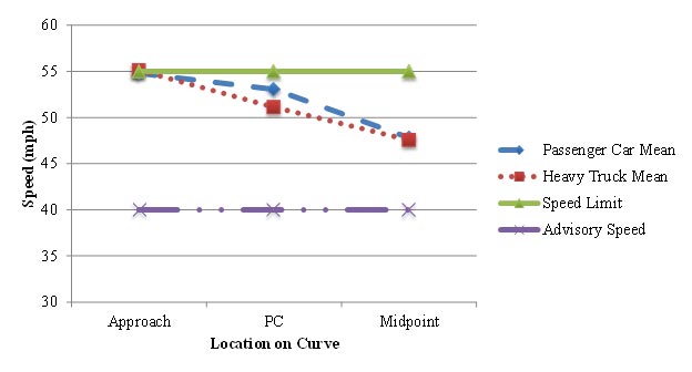
Figure 34. Graph. Graphical representation of speeds at the WV Route 32 treatment site.
Friction data were collected at eight locations at this study site, as described in the Friction Evaluation Methodology section. Table 10 shows the data-collection locations and the measurements that were taken for pavement macro-texture and pavement micro-texture. The pavement macro-texture was measured using the CT meter in accordance with ASTM E2517 to establish the MPD in millimeters. The frictional micro-texture characteristic of the sample surfaces was measured with the DF tester device according to the ASTM E1911 standard. The two complementary devices allowed the research team to calculate the IFI friction indices and subsequently translate the IFI numbers into predicted locked wheel friction numbers (Skid Number (SN) 65). Table 10 shows the SN 65 values based on the macro- and micro-texture measurements.
Table 10. WV Route 32 treatment site friction data.
Location |
PC +300 |
PC + 200 |
PC + 100 |
PC |
1/4 |
Mid |
3/4 |
PT |
CTM MPD |
0.750 |
0.790 |
0.943 |
0.977 |
0.930 |
0.987 |
0.940 |
0.980 |
DFT 20 |
0.530 |
0.595 |
0.495 |
0.490 |
0.395 |
0.480 |
0.385 |
0.400 |
SN 65 |
0.410 |
0.460 |
0.400 |
0.390 |
0.320 |
0.380 |
0.310 |
0.320 |
CTM = Circular Texture Meter
MPD = Mean Profile Depth
DFT = Dynamic Friction Meter
SN = Skid Number
PC = Point of Curvature
PT = Point of Tangent
As table 10 shows, the skid number at 40 mph is lower within the curve than before the curve, which was expected as a result of greater friction demand in the lateral direction when cornering. The research team collected encroachment data for 127 vehicles in the northbound direction and 132 vehicles in the southbound direction. Seventeen vehicles encroached onto the shoulder, and no vehicles crossed the centerline of the road in the northbound direction. Twelve vehicles crossed the centerline and 6 vehicles encroached onto the shoulder in the southbound direction. Braking maneuvers were also observed for the northbound vehicles. Because the camera was located at the PC, only vehicles braking within the curve were observed. At this site, 35 of the 127 vehicles were observed to brake within the curve for the northbound direction.
West Virginia Route 32 Comparison Site (C1 in Table 6)
Data were also collected at a comparison site approximately 1 mi south of the treatment site on WV Route 32 at the same time of the same day as the treatment site. The direction of travel was also south to north on a similar horizontal curve to the right. The radius of curve and the curve length, calculated using Google Earth™, were found to be 1,073.3 ft and 1,213.6 ft, respectively. The superelevation for this curve was 7.0 percent, and the vertical grade was -3.5 percent, based on manual field measurements with a digital slope meter. There was a small slope on the inside of the curve that limited horizontal sight distance along the curve, and there was a driveway inside the curve, approximately at the quarter-point between the PC and the PT. The PSL was 55 mph. As shown in figure 35, there was a reverse curve warning sign (W1-4) with a 50-mph advisory speed plaque (W13-1P). The travel lanes were 10 ft wide, and there was a 4-ft shoulder on both sides.
Speed data were collected 300 ft before the PC, at the PC, and at the midpoint of the curve. The research team placed the sensor in the opposing direction of travel at the midpoint of the curve to determine whether vehicles were present in the opposing lane. The camera was placed upstream of the PC (approximately 100 ft) to observe braking before and into the curve for northbound vehicles. Figure 35 shows a graphical layout of the horizontal curve along with the speed data- collection locations.
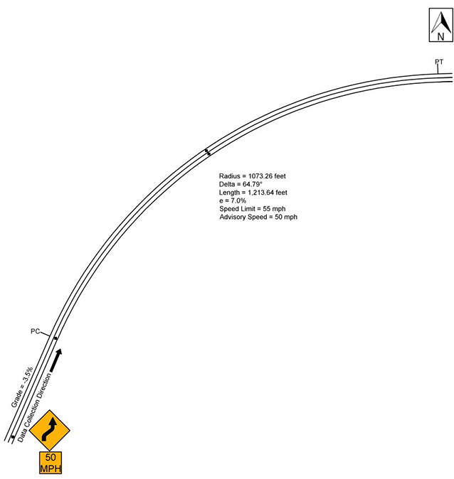
Figure 35. Diagram. Geometric layout of the WV Route 32 comparison site (not to scale).
Table 11 shows the speed data for the before period. A simple t-test was computed to compare the operating speeds at each data-collection location. For this comparison site, there were no statistically significant differences in speed measures.
Table 11. WV Route 32 comparison site before data.
| Speed Metric | Approach Speed |
Approach SD |
PC Speed |
PC SD |
Mid Speed |
Mid SD |
N |
| Passenger cars | 57.530 |
6.357 |
54.793 |
6.293 |
52.345 |
7.148 |
232 |
| Heavy trucks | 56.917 |
2.644 |
52.75 |
4.515 |
50.000 |
4.880 |
12 |
| Daytime passenger cars | 57.926 |
6.068 |
54.886 |
5.912 |
52.737 |
7.301 |
175 |
| Nighttime passenger cars | 56.917 |
7.114 |
54.446 |
7.444 |
51.107 |
6.627 |
56 |
| Opposed passenger cars | 58.581 |
5.870 |
54.774 |
5.812 |
52.452 |
7.348 |
31 |
| Unopposed passenger cars | 57.368 |
6.427 |
54.796 |
6.378 |
52.328 |
7.135 |
201 |
| Free-flow passenger cars | 57.623 |
6.381 |
54.912 |
6.387 |
52.265 |
7.402 |
204 |
| Non free-flow passenger cars | 56.857 |
6.246 |
53.929 |
5.591 |
52.929 |
4.981 |
28 |
Bold indicates
significance at the 95-percent confidence level (α=0.05)
SD = Standard Deviation
PC = Point of Curvature
N = Number of Observations
Figure 36 graphically shows the PSL, advisory speed limit, and the mean speeds for passenger cars and trucks along the WV Route 32 comparison section during the before period. As shown, the truck and passenger car mean speeds are similar across the section, but the heavy truck mean speed is consistently about 2 mph less than the passenger car mean speed. The deceleration rates appear to be very similar. The dispersion of speed at the midpoint of the curve is much greater for passenger cars than at the other locations, which leads to the 85th percentile being relatively stable from the approach to the midpoint of the curve. The mean acceleration rate from the PC to the midpoint of the curve was -0.434 ft/s (1.38) for passenger cars and -0.615 ft/s (0.700) for heavy trucks.
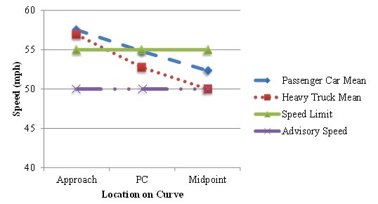
Figure 36. Graph. Graphical representation of speeds at the WV Route 32 comparison site.
The research team also collected friction data at eight locations within the comparison site. Table 12 presents the macro-texture, micro-texture, and SNs at the horizontal curve and approach locations. SNs within the curve were lower those on the approach tangent, which was expected because of the lateral friction demand by drivers traversing horizontal curves.
Table 12. WV Route 32 comparison site friction data.
| Location | PC +300 |
PC + 200 |
PC + 100 |
PC |
1/4 |
Mid |
3/4 |
PT |
| CTM MPD | 0.727 |
0.830 |
0.790 |
0.980 |
0.873 |
0.870 |
1.560 |
1.037 |
| DFT 20 | 0.480 |
0.515 |
0.500 |
0.450 |
0.445 |
0.450 |
0.395 |
0.525 |
| SN 65 | 0.380 |
0.410 |
0.400 |
0.360 |
0.360 |
0.360 |
0.280 |
0.420 |
CTM = Circular Texture Meter
MPD = Mean Profile Depth
DFT = Dynamic Friction Meter
SN = Skid Number
PC = Point of Curvature
PT = Point of Tangent
The research team collected encroachment data for 110 vehicles in the northbound direction and 129 vehicles in the southbound direction. Two vehicles encroached onto the shoulder, and no vehicles crossed the centerline in the northbound direction. Six vehicles crossed the centerline, and no vehicles encroached onto the shoulder in the southbound direction. Braking maneuvers were also observed for the northbound vehicles. Because the camera was located before the PC, vehicles braking before and within the curve were observed. At this site, 15 of the 110 vehicles were observed to brake before the curve and 10 of the 110 were observed to brake within the curve.
U.S. Route 33 Treatment Site (T2 in Table 6)
The second treatment site was located on U.S. Route 33 east of Harman, WV. The direction of travel for the data collection was in the eastbound direction. The radius of curve and the curve length, calculated using Google Earth™, were 209.97 ft and 539.22 ft, respectively. The superelevation for this curve was 6.0 percent, and the vertical grade was -8.0 percent. There was a substantial slope on the inside of the curve, which limited horizontal sight distance along the curve. The PSL was 55 mph. As figure 37 shows, there is a reverse turn warning sign (W1-3) with a 25 mph advisory speed plaque (W13-1P). The travel lanes were 11 ft wide, and there was a 4-ft shoulder on both sides.
Speed data were collected 300 ft before the PC, at the PC, and at the midpoint of the curve. The sensor was placed in the opposing direction of travel at the midpoint of the curve to determine whether vehicles were present in the opposing lane. In this case, there were two travel lanes in the westbound direction, and the sensor was placed in the left lane. The camera was placed upstream of the PC (approximately 200 ft) to allow for observation of braking before and into the curve for eastbound vehicles. Figure 37 shows the horizontal curve along with the speed data- collection locations.
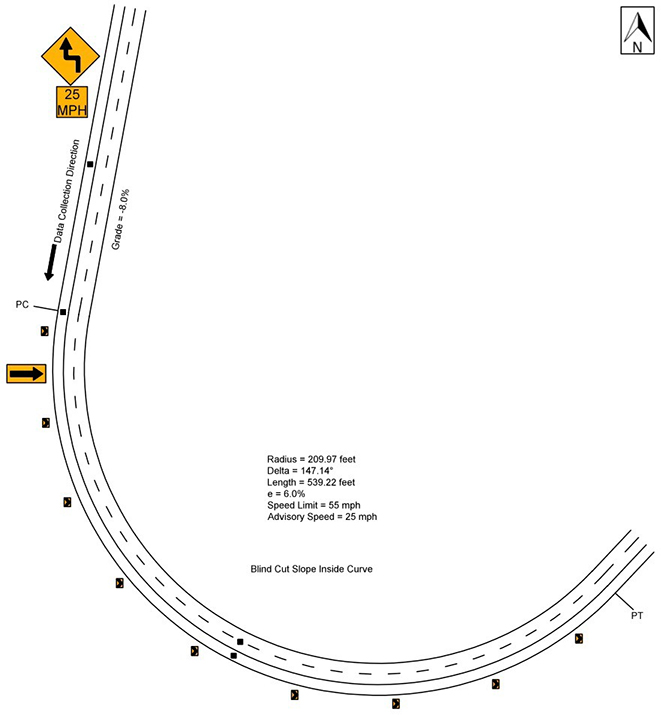
Figure 37. Diagram. Geometric layout of the U.S. Route 33 treatment site (not to scale).
Table 13 shows the speed data for the before period. The research team performed a simple t-test for each of these comparisons at each of the curve locations. Evaluation at this site showed statistically significant differences between passenger car and heavy truck speeds at all three locations. The difference was approximately 13 mph at the approach and 3.5 mph at the midpoint of the curve. Daytime speeds exceeded nighttime speeds for all locations, but the difference was only statistically significant at the PC. The relationship between free-flow speeds and non-free- flow speeds was inconsistent, and the difference was statistically significant at the PC.
Table 13. U.S. Route 33 treatment site before data.
| Speed Metric | Approach Speed |
Approach SD |
PC Speed |
PC SD |
Mid Speed |
Mid SD |
N |
| Passenger cars | 47.413 |
6.675 |
39.120 |
5.855 |
31.982 |
4.705 |
276 |
| Heavy trucks | 34.265 |
8.497 |
32.118 |
5.536 |
28.441 |
7.153 |
34 |
| Daytime passenger cars | 47.715 |
6.725 |
39.729 |
5.647 |
32.113 |
4.383 |
221 |
| Nighttime passenger cars | 46.200 |
6.384 |
36.673 |
6.086 |
31.455 |
5.843 |
55 |
| Opposed passenger cars | 47.970 |
7.760 |
38.788 |
6.637 |
31.982 |
4.705 |
33 |
| Unopposed passenger cars | 47.337 |
6.528 |
39.165 |
5.754 |
28.441 |
7.153 |
243 |
| Free-flow passenger cars | 47.332 |
6.747 |
38.817 |
5.656 |
32.127 |
4.709 |
229 |
| Non-free-flow passenger cars | 47.809 |
6.368 |
40.596 |
6.609 |
31.277 |
4.675 |
47 |
Bold indicates
significance at the 95-percent confidence level (α=0.05).
SD = Standard Deviation
PC = Point of Curvature
N = Number of Observations
Figure 38 graphically shows the PSL, advisory speed limit, and the mean speeds for passenger cars and trucks along the U.S. Route 33 treatment section during the before period. As shown, the passenger car speeds decelerate substantially from the approach to the middle of the curve. The heavy truck mean speeds are more aligned with the 15th percentile passenger car speed, but there is less deceleration for heavy vehicles than passenger cars at this site. The truck speeds are consistent with the advisory speed of 25 mph at the midpoint of the curve. The mean acceleration rate from the PC to the midpoint of the curve was found to be -1.58 ft/s (0.817) for passenger cars and -1.075 ft/s (0.887) for heavy trucks.
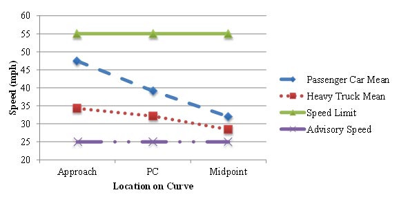
Figure 38. Graph. Graphical representation of speeds at the U.S. Route 33 treatment site.
Table 14 shows the macro-texture, micro-texture, and SNs for the U.S. Route 33 treatment site across the eight data-collection locations. The data show no discernible pattern because the friction and texture levels are fairly constant throughout the site.
Table 14. U.S. Route 33 treatment site friction data.
Location |
PC +300 |
PC + 200 |
PC + 100 |
PC |
1/4 |
Mid |
3/4 |
PT |
CTM MPD |
0.703 |
1.137 |
0.937 |
0.877 |
0.910 |
0.717 |
1.060 |
0.703 |
DFT 20 |
0.415 |
0.435 |
0.425 |
0.505 |
0.405 |
0.390 |
0.405 |
0.460 |
SN 65 |
0.330 |
0.340 |
0.340 |
0.400 |
0.330 |
0.320 |
0.320 |
0.360 |
CTM = Circular Texture Meter
MPD = Mean Profile Depth
DFT
= Dynamic Friction Meter
SN = Skid Number
PC = Point of Curvature
PT = Point of Tangent
Encroachment data were collected for 122 vehicles in the eastbound direction and 130 vehicles in the westbound direction. Six vehicles encroached onto the shoulder, and 15 vehicles crossed the centerline in the eastbound direction. Two vehicles crossed the centerline, and one vehicle encroached onto the shoulder in the westbound direction. Because there were two travel lanes in the westbound direction, it was observed that 48 vehicles crossed or straddled the broken line between the two lanes in the same direction. Braking maneuvers were also observed for the eastbound vehicles. Because the camera was located before the PC, vehicles braking before and within the curve were observed. At this site, 115 of the 122 vehicles were observed to brake before the curve, and 3 of the 122 vehicles were observed to brake within the curve.
U.S. Route 33 Comparison Site (C2 in Table 6)
Data for the U.S. Route 33 comparison were collected approximately 2 mi east of the treatment site. The direction of travel for the data collection was eastbound. The radius of curve and the curve length, calculated using Google Earth™, were 264.83 ft and 693.60 ft, respectively. The superelevation for this curve was 8.5 percent, and the vertical grade was -7.5 percent. There was a substantial cut-slope on the inside of the curve that limited horizontal sight distance along the curve. The PSL was 55 mph. As figure 39 shows, there was a reverse turn warning sign (W1-3) with a 25-mph advisory speed plaque (W13-1P). The travel lanes were 11 ft wide, and there was a 4-ft shoulder on both sides.
Speed data were collected 100 ft before the PC (because of the proximity of an adjacent horizontal curve), at the PC, and at the midpoint of the curve. The sensor in the opposing direction of travel was placed at the midpoint of the curve to whether vehicles were present in the opposing lane. The camera was placed upstream of the PC (approximately 200 ft) to allow observation of braking before and into the curve for eastbound vehicles. Figure 39 shows the horizontal curve along with the speed data-collection locations.
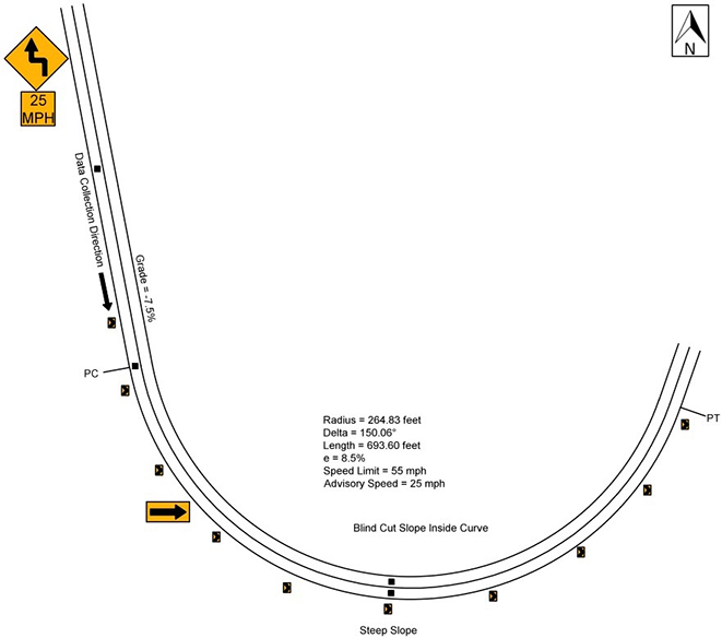
Figure 39. Diagram. Geometric layout of the U.S. Route 33 comparison site (not to scale).
Table 15 shows the speed data for the before period. The research team performed a simple t-test for each of the comparative measures at each of the curve locations. For this site, a statistically significant difference was found between passenger car and heavy truck speeds at all three locations. The difference was approximately 5.5 mph at the approach and PC locations, and 2.5 mph at the midpoint of the curve. The daytime speeds were greater than the nighttime speeds at all three locations, but the difference was only statistically significant at the PC. The free-flow speeds were greater than the non-free-flow speeds at all locations, but the difference was not statistically significant at the midpoint of the curve.
Table 15. U.S. Route 33 comparison site before data.
| Speed Metric | Approach Speed |
Approach SD |
PC Speed |
PC SD |
Mid Speed |
Mid SD |
N |
| Passenger cars | 43.027 |
5.966 |
38.608 |
6.566 |
35.814 |
6.528 |
263 |
| Heavy trucks | 37.564 |
8.012 |
32.974 |
7.354 |
33.128 |
5.908 |
39 |
| Daytime passenger cars | 43.376 |
5.804 |
39.168 |
6.362 |
36.056 |
6.633 |
197 |
| Nighttime passenger cars | 41.985 |
6.360 |
36.939 |
6.926 |
35.091 |
6.196 |
66 |
| Opposed passenger cars | 43.377 |
6.404 |
38.434 |
7.680 |
35.547 |
6.444 |
53 |
| Unopposed passenger cars | 42.938 |
5.864 |
38.652 |
6.274 |
35.881 |
6.562 |
210 |
| Free-flow passenger cars | 43.404 |
5.866 |
39.207 |
6.289 |
35.914 |
6.528 |
208 |
| Non-free-flow passenger cars | 41.600 |
6.181 |
36.345 |
7.142 |
35.436 |
6.786 |
55 |
Bold indicates
significance at the 95-percent confidence level (α=0.05).
SD = Standard Deviation
PC = Point of Curve
N = Number of Observations
Figure 40 graphically shows the PSL, advisory speed limit, and the mean speeds for passenger cars and trucks along the U.S. Route 33 comparison section during the before period. As was the case at the treatment site, the mean speed for passenger cars decreased across the study section at a greater rate than the heavy trucks. However, the mean heavy truck speed stabilized at about 33 mph, which is 8 mph greater than the advisory speed. The 85th percentile speed for passenger cars was approximately the PSL (55 mph) at the approach and decreased to about 49 mph at the midpoint of the curve. The 15th percentile speed was approximately the advisory speed of 25 mph at the midpoint of the curve. There does not appear to be a relationship between passenger car speeds and heavy truck speeds at this site. The mean acceleration rate from the PC to the midpoint of the curve was found to be -0.679 ft/s (1.664) for passenger cars and -0.262 ft/s (1.468) for heavy trucks.
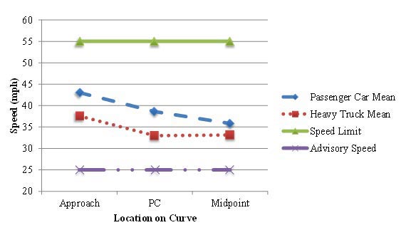
Figure 40. Graph. Graphical representation of speeds at the U.S. Route 33 comparison site.
Table 16 shows the macro-texture, micro-texture, and SNs for the U.S. Route 33 comparison site across the seven data-collection locations. It is clear from the data that both the macro-texture and micro-texture are very low at this site. This leads to a range of SNs from a low of 0.26 at the three-quarter point of the curve to a high of 0.34 at the PC. Similar to the treatment site, the comparison site is located on a very steep grade (approximately 8 percent). The steep grade creates the need for braking throughout the entire treatment and comparison sites, which is likely the reason that the pavement texture is consistent, but low, throughout the study site.
Table 16. U.S. Route 33 comparison site friction data.
Location |
PC + 200 |
PC + 100 |
PC |
1/4 |
Mid |
3/4 |
PT |
CTM MPD |
0.463 |
0.530 |
0.547 |
0.420 |
0.350 |
0.327 |
0.430 |
DFT 20 |
0.355 |
0.400 |
0.450 |
0.360 |
0.400 |
0.365 |
0.380 |
SN 65 |
0.28 |
0.31 |
0.34 |
0.28 |
0.28 |
0.26 |
0.29 |
CTM = Circular Texture Meter
MPD = Mean Profile Depth
DFT
= Dynamic Friction Meter
SN = Skid Number
PC = Point of Curvature
PT = Point of Tangent
The research team collected encroachment data for 89 vehicles in the eastbound direction and 92 vehicles in the westbound direction. Four vehicles encroached onto the shoulder, and 10 vehicles crossed the centerline in the eastbound direction. Five vehicles crossed the centerline, and 12 vehicles encroached onto the shoulder in the westbound direction. Braking maneuvers were also observed for the eastbound vehicles. Because the camera was located before the PC, vehicles braking before and within the curve were observed. At this site, 85 of the 89 vehicles were observed to brake before the curve, and 2 of the 89 vehicles were observed to brake within the curve.
U.S. Route 219 Treatment Site A—Mile Marker 6.32 (T3 in Table 6)
Data at treatment site A on U.S. Route 219 were collected in the northbound direction of travel. The radius of curve and the curve length, calculated using Google Earth™, were 605.08 ft and 753.82 ft, respectively. The superelevation for this curve was 11 percent, and the vertical grade was -2.0 percent. There was a roadside slope on the inside of the curve that limited horizontal sight distance along the curve. The PSL was 55 mph. As figure 41 shows, there was a warning sign (W1-2) of a curve to the right with a 30 mph advisory speed plaque (W13-1P). The travel lanes were 10 ft wide, and there was a 1-ft paved shoulder on both sides.
Speed data were collected 300 ft before the PC, at the PC, and at the midpoint of the curve. The sensor in the opposing direction of travel was placed at the midpoint of the curve to determine whether vehicles were present in the opposing lane. The camera was placed upstream of the PC (approximately 200 ft) to allow observation of braking before and into the curve for northbound vehicles. Figure 41 shows a graphical layout of the horizontal curve along with the speed data- collection locations.
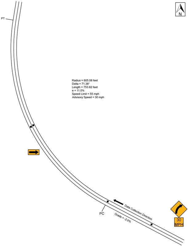
Figure 41. Diagram. Geometric layout of the U.S. Route 219 treatment A site (not to scale).
Table 17 presents the speed data for the before period. The research team completed a simple t-test for each of the speed measures at each of the curve locations. For this site, passenger car speeds were greater than the heavy truck speeds at all three locations. The difference was statistically significant at the approach location only. Daytime and nighttime speeds were statistically significant at the approach; however, there were only 14 vehicles observed in the nighttime period. At the approach and PC, the nighttime speeds were greater than the daytime speeds. The daytime speeds were greater (although insignificantly) that nighttime speeds at the midpoint of the curve.
Table 17. U.S. Route 219 treatment A site before data.
| Speed Metric | Approach Speed |
Approach SD |
PC Speed |
PC SD |
Mid Speed |
Mid SD |
N |
| Passenger cars | 48.125 |
6.058 |
46.397 |
6.062 |
36.294 |
7.532 |
136 |
| Heavy trucks | 43.944 |
5.826 |
45.222 |
5.287 |
34.389 |
4.629 |
18 |
| Daytime passenger cars | 47.893 |
6.172 |
46.336 |
6.191 |
36.434 |
7.356 |
122 |
| Nighttime passenger cars | 50.143 |
4.655 |
46.929 |
4.953 |
35.071 |
9.144 |
14 |
| Opposed passenger cars | 46.889 |
6.615 |
46.167 |
6.947 |
37.667 |
9.172 |
18 |
| Unopposed passenger cars | 48.314 |
5.977 |
46.432 |
5.948 |
36.085 |
7.273 |
118 |
| Free-flow passenger cars | 48.383 |
6.059 |
46.600 |
6.039 |
36.565 |
7.542 |
115 |
| Non-free-flow passenger cars | 46.714 |
6.282 |
45.286 |
6.214 |
34.810 |
7.481 |
21 |
Bold indicates
significance at the 95-percent confidence level (α=0.05).
SD = Standard Deviation
PC = Point of Curvature
N = Number of Observations
Figure 42 graphically shows the PSL, advisory speed limit, and the mean speeds for passenger cars and trucks along U.S. Route 219 treatment site A during the before period. The figure shows that mean speeds for both heavy trucks and passenger cars remain relatively stable from the approach to the PC, but decrease substantially from the PC to the midpoint of the curve. At this site, it is clear that the mean speeds for both passenger cars and heavy trucks are similar across the study segment. The mean speeds are approximately 5 mph greater than the advisory speed of 30 mph at the midpoint of the curve. It is also clear that the dispersion of speed decreases substantially within the horizontal curve. The mean acceleration rate from the PC to the midpoint of the horizontal curve was -3.178 ft/s (2.959) for passenger cars and -3.042 ft/s (2.811) for heavy trucks.
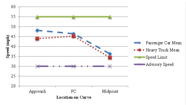
Figure 42. Graph. Graphical representation of speeds at the U.S. Route 219 treatment A site.
Table 18 shows the macro-texture, micro-texture, and SNs for the U.S. 219 treatment A site across the eight data-collection locations. From the table, it is clear that the mean profile depth is much greater across the entire site than the other data-collection sites. Greater mean-profile depth is associated with a lower SN. Conversely, the micro-texture friction is higher than most sites. The SN appears to be fairly constant from the approach throughout the horizontal curve.
Table 18. U.S. Route 219 treatment A site friction data.
| Location | PC +300 |
PC + 200 |
PC + 100 |
PC |
1/4 |
Mid |
3/4 |
PT |
| CTM MPD | 1.407 |
1.417 |
1.407 |
1.277 |
0.890 |
0.950 |
1.093 |
1.140 |
| DFT 20 | 0.500 |
0.490 |
0.525 |
0.530 |
0.505 |
0.465 |
0.585 |
0.545 |
| SN 65 | 0.380 |
0.370 |
0.360 |
0.400 |
0.360 |
0.380 |
0.370 |
0.400 |
CTM = Circular Texture Meter
MPD = Mean Profile Depth
DFT
= Dynamic Friction Meter
SN = Skid Number
PC = Point of Curvature
PT = Point of Tangent
Encroachment data were collected for 77 vehicles in the northbound direction and 92 vehicles in the southbound direction. Two vehicles encroached onto the shoulder, and no vehicles crossed the centerline in the northbound direction. Six vehicles crossed the centerline, and three vehicles encroached onto the shoulder in the southbound direction. Braking maneuvers were also observed for the northbound vehicles. Because the camera was located before the PC, vehicles braking before and within the curve were observed. At this site, 56 of the 77 vehicles were observed braking before the curve, and 12 of the 77 vehicles were observed braking within the curve.
U.S. Route 219 Treatment Site B―Mile Marker 5.81 (T4 in Table 6)
The research team also collected at a second treatment site along U.S. Route 219. The direction of travel for the data collection was northbound. The radius of curve and the curve length, calculated using Google Earth™, were 272.85 ft and 673.42 ft, respectively. The superelevation for this curve was 12 percent, and the vertical grade was -3.0 percent. There was a roadside slope on the inside of the curve that limited horizontal sight distance along the curve. The travel lanes were 10.5 ft wide, and there was a 1-ft paved shoulder on both sides. The PSL is 55 mph. As Figure 44 shows, there was a warning sign (W1-2) of a curve to the right with a 25-mph advisory speed plaque (W13-1P).
Speed data were collected 300 ft before the PC, at the PC, and at the midpoint of the curve. The sensor in the opposing direction of travel was placed at the midpoint of the curve to determine whether vehicles were present in the opposing lane. The camera was placed upstream of the PC (approximately 200 ft) to observe braking before and into the curve for northbound vehicles. Figure 43 shows the layout of the horizontal curve along with the speed data-collection locations.
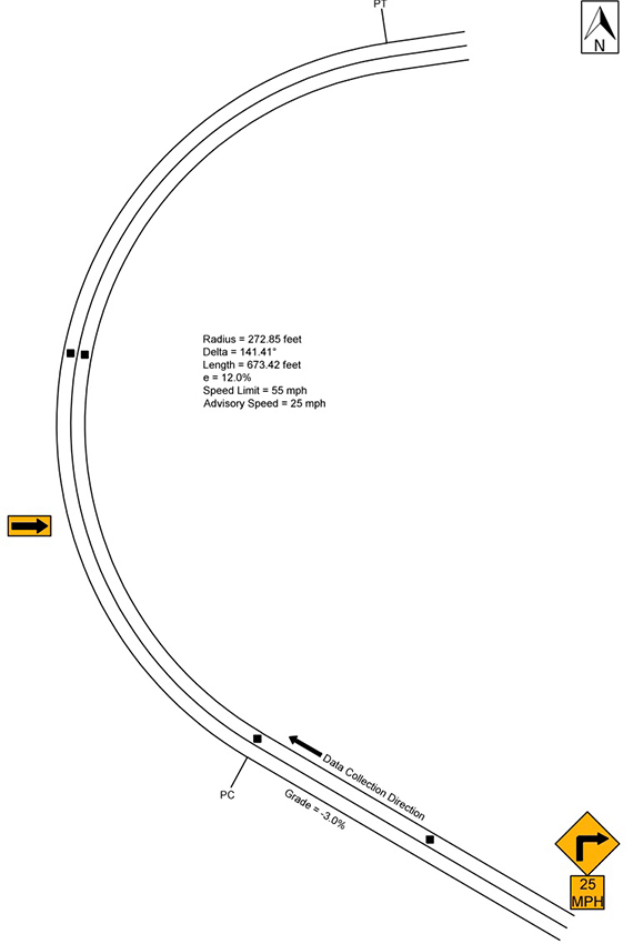
Figure 43. Diagram. Geometric layout of the U.S. Route 219 treatment B site (not to scale).
Table 19 presents speed data for the before period. A simple t-test was computed for each of these comparisons at each of the curve locations. For this site, passenger car speeds were greater than the heavy truck speeds at all three locations. The difference was statistically significant at the PC only. The unopposed passenger car speeds were greater than the opposed passenger car speeds at all three locations. Free-flow speeds were statistically different than non-free-flow speeds at the PC only.
Table 19. U.S. Route 219 treatment B site before data.
| Speed Metric | Approach Speed |
Approach SD |
PC Speed |
PC SD |
Mid Speed |
Mid SD |
N |
| Passenger cars | 48.661 |
8.304 |
44.724 |
6.720 |
34.622 |
6.285 |
127 |
| Heavy trucks | 46.684 |
7.616 |
39.263 |
6.145 |
33.474 |
4.823 |
19 |
| Daytime passenger cars | 48.848 |
8.082 |
44.857 |
6.881 |
34.464 |
6.373 |
112 |
| Nighttime passenger cars | 47.267 |
10.018 |
43.733 |
5.457 |
35.800 |
5.647 |
15 |
| Opposed passenger cars | 46.769 |
5.085 |
44.615 |
4.445 |
33.154 |
4.616 |
13 |
| Unopposed passenger cars | 48.877 |
8.584 |
44.737 |
6.946 |
34.789 |
6.443 |
127 |
| Free-flow passenger cars | 48.413 |
8.647 |
45.298 |
6.914 |
34.712 |
6.406 |
104 |
| Non-free-flow passenger cars | 49.783 |
6.578 |
42.130 |
5.120 |
34.217 |
5.823 |
23 |
Bold indicates
significance at the 95-percent confidence level (α=0.05).
SD = Standard Deviation
PC = Point of Curve
N = Number of Observations
Figure 44 graphically shows the PSL, advisory speed limit, and the mean speeds for passenger cars and trucks along U.S. Route 219 treatment site B during the before period. The figure shows that passenger cars decelerate at a much greater rate within the horizontal curve compared with the approach to the horizontal curve. Heavy trucks appear to have a more constant deceleration from the approach to the midpoint of the horizontal curve, which explains the significant difference at the PC location. Mean speeds are about 7 mph less than the PSL at the approach and about 10 mph greater than the advisory speed at the midpoint of the horizontal curve. The 15th percentile speed is approximately equal to the advisory speed at the midpoint of the horizontal curve. The mean acceleration rate from the PC to the midpoint of the curve was - 2.603 ft/s (2.064) for passenger cars and -1.645 ft/s (1.53) for heavy vehicles.
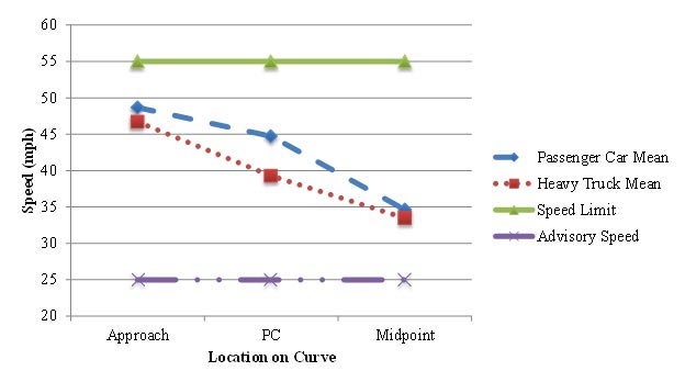
Figure 44. Graph. Graphical representation of speeds at the U.S. Route 219 treatment B site.
Table 20 shows the macro-texture, micro-texture, and SNs for the U.S. Route 219 treatment B site across the eight data-collection locations. Again, there is no discernible pattern of the SN from the approach to the end of the site, but the SN is pretty high compared with many of the other sites. The mean-profile depth is small (ranging from 0.493 to 0.823), and the micro-texture friction is high (ranging from 0.465 to 0.585).
Table 20. U.S. Route 219 treatment B site friction data.
Location |
PC +300 |
PC + 200 |
PC + 100 |
PC |
1/4 |
Mid |
3/4 |
PT |
CTM MPD |
0.493 |
0.493 |
0.647 |
0.680 |
0.823 |
0.570 |
0.643 |
0.573 |
DFT 20 |
0.535 |
0.560 |
0.525 |
0.530 |
0.505 |
0.465 |
0.585 |
0.545 |
SN 65 |
0.380 |
0.400 |
0.400 |
0.410 |
0.400 |
0.350 |
0.440 |
0.400 |
CTM = Circular Texture Meter
MPD = Mean Profile Depth
DFT
= Dynamic Friction Meter
SN = Skid Number
PC = Point of Curvature
PT = Point of Tangent
The research team collected encroachment data for 61 vehicles in the northbound direction and 61 vehicles in the southbound direction. Ten vehicles encroached onto the shoulder, and 10 vehicles crossed the centerline in the northbound direction. Twelve vehicles crossed the centerline, and 2 vehicles encroached onto the shoulder in the southbound direction. Braking maneuvers were also observed for the northbound vehicles. Because the camera was located before the PC, vehicles braking before and within the curve were observed. At this site, 31 of the 61 vehicles were observed braking before the curve, and 20 of the 61 vehicles were observed braking within the curve.
U.S. Route 219 Comparison Site (C3/C4 in Table 6)
The U.S. Route 219 comparison site was located approximately 5 mi north of the two treatment sites on the same route. The direction of travel for the data collection was northbound. The curve radius and the curve length, calculated using Google Earth™, were 544.57 ft and 826.91 ft, respectively. The superelevation for this curve was 12 percent, and the vertical grade was -6.5 percent. The PSL was 55 mph. As figure 45 shows, there was a reverse curve warning sign (W1-4) with a 30-mph advisory speed plaque (W13-1P). The travel lanes were 11 ft wide, and there was no paved shoulder.
Speed data were collected 100 ft before the PC (because of an adjacent horizontal curve), at the PC, and at the midpoint of the curve. The research team placed the sensor in the opposing direction of travel at the midpoint of the curve to determine whether vehicles were present in the opposing lane. The camera was placed at the PC to observe braking into the curve for northbound vehicles. Figure 45 shows a layout of the horizontal curve along with the speed data- collection locations.
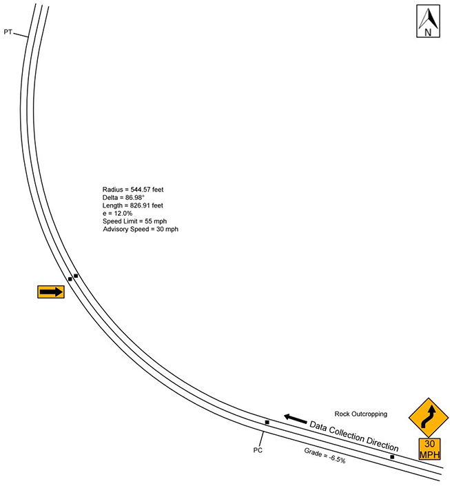
Figure 45. Diagram. Geometric layout of the U.S. Route 219 comparison site (not to scale).
Table 21 presents the speed data for the before period. The research team computed a simple t-test for each of the speed measures at each of the curve locations. The passenger car speeds were greater than the heavy truck speeds at all three locations. This difference was statistically significant at all three locations, even with only 79 and 13 passenger car and truck speed observations, respectively. The daytime speeds were greater than the nighttime speeds at all three sites. This difference was not statistically significant at any site, likely owing to the small sample size. The opposed passenger car speeds were greater than the unopposed passenger car speeds at every site, and were statistically significant at the approach. The free-flow speeds were greater than the non-free-flow speeds at every site, but not statistically significant at any location.
Table 21. U.S. Route 219 comparison site before data.
| Speed Metric | Approach Speed |
Approach SD |
PC Speed |
PC SD |
Mid Speed |
Mid SD |
N |
| Passenger cars | 44.506 |
6.961 |
42.025 |
6.653 |
41.152 |
5.371 |
79 |
| Heavy trucks | 39.154 |
7.186 |
38.154 |
5.886 |
36.000 |
6.506 |
13 |
| Daytime passenger cars | 44.647 |
6.083 |
42.176 |
5.122 |
41.426 |
4.566 |
68 |
| Nighttime passenger cars | 43.634 |
11.360 |
41.091 |
12.973 |
39.455 |
9.038 |
11 |
| Opposed passenger cars | 46.000 |
4.219 |
43.273 |
5.442 |
42.909 |
5.594 |
11 |
| Unopposed passenger cars | 43.444 |
7.482 |
41.235 |
6.799 |
40.086 |
5.771 |
81 |
| Free-flow passenger cars | 44.714 |
7.051 |
42.100 |
6.740 |
41.157 |
5.468 |
70 |
| Non free-flow passenger cars | 42.889 |
6.353 |
41.444 |
6.267 |
41.111 |
4.833 |
9 |
Bold indicates significance at the 95-percent confidence level (α =0.05).
SD = Standard Deviation
PC = Point of Curvature
N = Number of Observations
Figure 46 graphically shows the PSL, advisory speed limit, and the mean speeds for passenger cars and trucks along the U.S. Route 219 comparison site during the before period. The passenger car and heavy truck speeds remain fairly constant from the approach to the midpoint of the horizontal curve. This is likely because this horizontal curve is in the middle of several horizontal curves with no long tangent sections between. The mean passenger car speed was approximately 12 mph greater than the advisory speed, and the heavy truck speed was approximately 10 mph greater. The 85th percentile operating speed was approximately equal to the PSL (55 mph). The mean acceleration rate from the PC to the midpoint of the curve was -0.213 ft/s (1.201) for passenger cars and -0.157 ft/s (1.627) for heavy trucks.
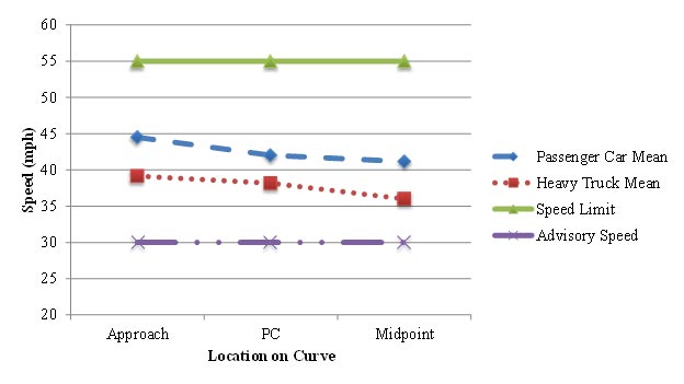
Figure 46. Graph. Graphical representation of speeds at the U.S. Route 219 comparison site.
Table 22 shows the macro-texture, micro-texture, and SNs for the U.S. Route 219 comparison site across the six data-collection locations. As the table shows, the SN is quite low across the site and is somewhat uniform from the approach to the end of the horizontal curve. Again, the site is on a fairly substantial grade (about 6.5 percent downhill), which may contribute to increased longitudinal friction as a result of braking.
Table 22. U.S. Route 219 comparison site friction data.
| Location | PC + 100 |
PC |
1/4 |
Mid |
3/4 |
PT |
| CTM MPD | 0.650 |
0.760 |
0.457 |
0.520 |
0.610 |
0.683 |
| DFT 20 | 0.390 |
0.395 |
0.385 |
0.390 |
0.410 |
0.390 |
| SN 65 | 0.310 |
0.320 |
0.290 |
0.300 |
0.330 |
0.320 |
CTM = Circular Texture Meter
MPD = Mean Profile Depth
DFT
= Dynamic Friction Meter
SN = Skid Number
PC = Point of Curvature
PT = Point of Tangent
Encroachment data were collected for 49 vehicles in the northbound direction and 60 vehicles in the southbound direction. Eight vehicles encroached onto the shoulder, and no vehicles crossed the centerline in the northbound direction. Twenty vehicles crossed the centerline, and 3 vehicles encroached onto the shoulder in the southbound direction. Braking maneuvers were also observed for the northbound vehicles. Because the camera was located at the PC, vehicles braking maneuvers within the curve were observed. At this site, 47 of the 49 vehicles were observed to brake within the curve.
COMPARISON OF BEFORE AND AFTER PERIOD DATA
The HFST was applied to the four treatment site locations in June 2012, and the research team observed speed, encroachment, and braking maneuvers in August 2012. The second after period data-collection effort was completed in June 2013, and included speed, encroachment, and braking maneuver field measurements and observation. This section of the report describes the differences found between the before and after conditions at the treatment sites, as well as the comparison sites. If significant differences were found from the before to after condition at the comparison sites, then those differences were considered in the analysis of the treatment sites.
As described in the data collection and analysis methods section above, the research team excluded all vehicles that were not passenger cars and that were not considered free-flow vehicles from the analysis database. The data analysis files also included indicators for when vehicles were present opposite to the travel lane where the operational evaluation was being conducted. The mean speed, change in mean speed between the PC and midpoint of the curve, percentage of vehicles exceeding the PSL, encroachment, and friction analysis results are all included in this section of the report.
West Virginia Route 32 (Treatment and Comparison Site)
Table 23 shows the before and after mean speeds and speed deviations for the treatment and comparison sites on WV Route 32. The table shows the values for both passenger cars and heavy trucks at the approach, PC, and curve midpoint. The mean and SDs are given for free-flow vehicles with no opposing vehicles in the opposite direction because very few vehicles were present in the opposing lane during the analysis period (see before data period data summary above) and because these mean speeds were seldom statistically different in the before period data analysis. Only daytime speeds were reported for comparison in the before and after periods because too few nighttime observations were available or because passenger car and truck speeds seldom varied in the before period analysis. As table 23 shows, there was no statistically significant change in speed measures for the comparison site from the before to the first after period. However, significant reductions in speed were found at the PC and curve midpoints for passenger cars at the treatment site. In both cases, the reduction was approximately 1.5 mph. The midpoint speed was found to be significantly lower for heavy trucks, by approximately 8 mph, in the first after period when compared with the before period, but this was likely the result of the very small number of trucks included in the sample. When comparing the second after period to the first after period, the mean truck speeds increased to levels similar to the before period.
There was a significant reduction in speed for passenger cars at the approach point in the second after period, when compared with the before period, at the treatment site. However, there was also a significant reduction at the approach point for the comparison site. When taking this reduction into account, the reduction in speed for the treatment site was no longer statistically significant. The mean speed of passenger cars at the PC and curve midpoint increased slightly in the second after period, but they were still less than the before period. There was a 4.2-mph reduction in truck speed at the approach of the treatment site, but this reduction did not continue through the curve. There was also a statistically significant increase in truck speeds at the curve midpoint in the second after period compared with the first. The increase was approximately 6.9 mph, but the speed was still 1.3 mph lower than the before period. The truck speed at the midpoint during the first after period was low when compared with the before and second after period, but there were 12 or fewer trucks in each observation period.
Table 23. Operating speeds at WV Route 32 sites before and after treatment.
| Speed Metric | Approach Speed |
Approach SD |
PC Speed |
PC SD |
Mid Speed |
Mid SD |
N |
| Treatment PCs before | 55.216 |
7.3 |
53.743 |
6.283 |
48.054 |
5.639 |
167 |
| Treatment PCs 1st after | 54.166 |
7.959 |
52.337 |
7.343 |
46.554 |
5.126 |
175 |
| Treatment PCs 2nd after | 53.111 |
8.447 |
52.849 |
6.645 |
47.633 |
7.212 |
199 |
| Treatment trucks before | 56.50 |
3.987 |
51.50 |
5.089 |
49.833 |
4.622 |
6 |
| Treatment trucks after | 55.125 |
3.227 |
50.50 |
5.855 |
41.625 |
4.658 |
8 |
| Treatment trucks 2nd after | 52.333 |
6.443 |
51.417 |
5.384 |
48.50 |
3.477 |
12 |
| Comparison PCs before | 57.839 |
6.04 |
55.04 |
6.046 |
52.758 |
7.617 |
124 |
| Comparison PCs 1st after | 57.443 |
5.317 |
54.584 |
5.057 |
52.227 |
5.587 |
185 |
| Comparison PCs 2nd after | 56.504 |
6.315 |
55.417 |
6.923 |
52.483 |
6.06 |
240 |
| Comparison trucks before | 56.429 |
2.992 |
53.857 |
2.734 |
49.429 |
3.823 |
7 |
| Comparison trucks 1st after | 57.889 |
8.023 |
52.556 |
5.94 |
50.667 |
5.148 |
9 |
| Comparison trucks 2nd after | 54.375 |
6.811 |
51.938 |
6.708 |
49.25 |
3.474 |
16 |
Bold indicates
significance at the 95-percent confidence level (α =0.05) when comparing either after period to the
before period.
Italics indicates significance at the 95-percent confidence level (α =0.05) between the 1st and 2nd after periods.
Underline indicates that, when accounting for the speed change at the comparison site, the change in the speed at
the treatment site was not statistically significant at the 95-percent confidence level (α = 0.05).
SD = Standard Deviation
PC = Point of Curvature
N = Number of Observations
Figure 47 and figure 48 show graphical representations of the speed profiles for the WV Route 32 treatment and comparison sites, respectively. The general shape of the speed profiles for the three collection periods remained relatively similar.
Passenger Car Operating Speeds
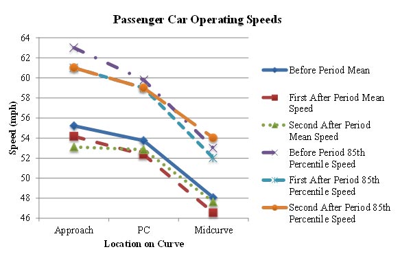
Figure 47. Graph. WV Route 32 treatment site operating speeds (PSL = 55 mph).
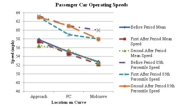
Figure 48. Graph. WV Route 32 comparison site operating speeds (PSL = 55 mph).
U.S. Route 33 (Treatment and Comparison Site)
Table 24 shows the before and after mean operating speeds for the treatment and comparison sites on U.S. Route 33. Again, there was no statistically significant change in mean speeds for both passenger cars and heavy trucks at the comparison from the before period to the first after period. The difference in mean speed for passenger cars between the before treatment application and first after treatment application were statistically significant at all three data-collection points. This difference shows reduced speed from the before to the after period at the treatment location. The change was approximately 1.3 mph at the approach and PC locations, and 1.7 mph at the midpoint of the curve. Passenger car speeds decreased by only 0.4 mph at the midpoint after considering passenger cars entered the curve by approximately 1.3 mph slower in the first after period. For heavy trucks, there was a statistically significant reduction in speed of 3.5 mph in the first after period at the PC.
Table 24 shows that mean speed for passenger cars significantly increased at the approach point by approximately 2.5 mph in the second after period compared with the first after period at the treatment site. Although not significant, the speed increase was approximately 1.2 mph at the approach point from the before period to the second after period. The significant increase in speed in the second after period continued through the PC location, where the increase was approximately 1.8 mph relative to the before period and 3.1 mph relative to the first after period. Passenger car speeds were significantly reduced in the second after period when compared with the before period at the comparison site, at the approach point and the PC, by approximately 1.3 mph and 1.4 mph, respectively. This reduction in speeds at the comparison site increases the significance of the increase in speeds at the approach point and PC at the treatment site. Passenger car mean speeds were significantly lower at the curve midpoint by approximately 2.2 mph, in the second after period, not taking into account the speed reduction at the comparison site. However, speeds were also significantly reduced at the midpoint of the comparison site by approximately 1.7 mph. When taking this reduction into account, the speed reduction at the curve midpoint of the treatment site was no longer statistically significant. As with the WV Route 32 site, the high-friction surface had no long-term effect on passenger car mean operating speeds at the curve midpoint of the U.S. Route 33 treatment site. However, there was a statistically significant speed reduction at both the PC and midpoint for trucks in the second after period.
Table 24. Operating speeds at U.S. Route 33 before and after treatment.
| Speed Metric | Approach Speed |
Approach SD |
PC Speed |
PC SD |
Mid Speed |
Mid SD |
N |
| Treatment PCs before | 47.608 |
6.538 |
39.544 |
5.346 |
32.367 |
4.571 |
158 |
| Treatment PCs 1st after | 46.301 |
7.512 |
38.245 |
5.771 |
30.614 |
3.791 |
163 |
| Treatment PCs 2nd after | 48.769 |
7.723 |
41.336 |
7.199 |
30.154 |
5.024 |
143 |
| Treatment trucks before | 34.158 |
7.762 |
32.368 |
3.7 |
27.263 |
4.188 |
19 |
| Treatment trucks 1st after | 33.50 |
11.329 |
28.833 |
8.855 |
27.167 |
4.967 |
24 |
| Treatment trucks 2nd after | 30.905 |
9.049 |
27.476 |
7.593 |
24.048 |
5.661 |
21 |
| Comparison PCs before | 43.661 |
5.812 |
39.347 |
6.318 |
36.169 |
6.786 |
118 |
| Comparison PCs 1st after | 42.865 |
5.372 |
38.361 |
5.055 |
35.459 |
6.086 |
133 |
| Comparison PCs 2nd after | 42.366 |
6.462 |
37.93 |
5.812 |
34.443 |
5.445 |
142 |
| Comparison trucks before | 39.214 |
5.409 |
35.286 |
5.045 |
32.00 |
5.698 |
14 |
| Comparison trucks 1st after | 36.621 |
8.918 |
32.897 |
8.461 |
31.517 |
7.41 |
29 |
| Comparison trucks 2nd after | 36.80 |
5.569 |
34.70 |
4.921 |
32.55 |
5.781 |
20 |
Bold indicates
significance at the 95-percent confidence level (α =0.05) when comparing either after period to the
before period.
Italics indicates significance at the 95-percent confidence level (α =0.05) between the 1st and 2nd after periods.
Underline indicates that, when accounting for the speed change at the comparison site, the change in the speed at
the treatment site was not statistically significant at the 95-percent confidence level (α = 0.05).
SD = Standard Deviation
PC = Point of Curvature
N = Number of Observations
Figure 49 and figure 50 show graphical representations of the speed profiles for the U.S. Route 33 treatment and comparison sites, respectively. The general shape of the speed profiles for the three collection periods remained relatively similar.
Passenger Car Operating Speeds
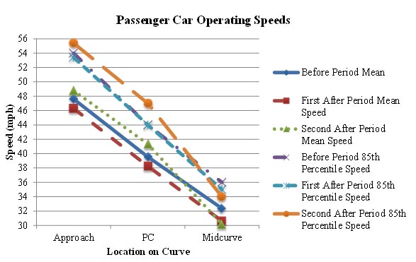
Figure 49. Graph. U.S. Route 33 treatment site operating speeds (PSL = 55 mph).
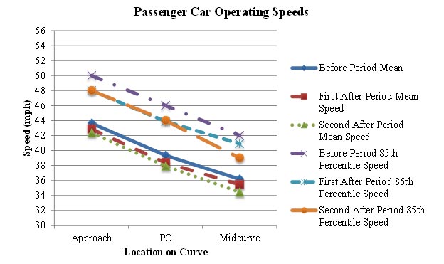
Figure 50. Graph. U.S. Route 33 comparison site operating speeds (PSL = 55 mph).
U.S. Route 219 (Treatment and Comparison Site)
Table 25 shows the mean speeds for passenger cars and heavy trucks for the treatment and comparison sites on U.S. Route 219. For these sites, there was a statistically significant increase in mean speed from the before period to the first after period at all three data-collection locations at the comparison site. This result was expected because the roadway was slightly damp in the before period. The data at the comparison site showed that approach and PC mean speeds increased by about 2.2 mph in the first after period relative to the before period. At the midcurve location, the mean speed increased by 2.7 mph when comparing the first after period with the before period. Without accounting for this change, the PC mean speed was significantly lower in the first after period relative to the before period at the MM 6.32 location, while the midpoint curve mean speed is significantly higher in the first after period relative to the before period. However, when taking the increase in speed at the comparison site into account, the speed increase at the curve midpoint of the first treatment site (MM 6.32) is no longer statistically significant. However, when accounting for the statistically significant reduction in the mean speed at the PC location, the PC mean speed reduction for passenger cars at the treatment site was approximately 4.8 mph, which was statistically significant. Passenger car speeds also increased, between the before period and first after period, at the second treatment site (MM 5.81), at the approach point and the midpoint of the curve. The speed increase was approximately 2.3 mph at both data-collection points. However, neither of these mean speed increases was statistically significant when considering the speed increases at the comparison site.
There were statistically significant changes at all three data-collection points at the comparison site in the second after period for passenger cars. There was a statistically significant increase in mean speed at the approach point between the before and second after periods, which was approximately 3.7 mph. There was also a statistically significant reduction in speed at the PC when comparing the second after period with the before period. There was no significant difference in speed at the midpoint of the curve between the second after and before periods. However, there was a statistically significant reduction in speed at the PC and curve midpoint between the first and second after periods. The speed reductions were approximately 4.6 mph at the PC and 2.7 mph at the curve midpoint.
Table 25 shows a significant speed reduction at the PC of the first treatment site (MM 6.32) in the second after period. This significant reduction was approximately 4 mph when compared with the before period and 1.4 mph when compared with the first after period. There was also a statistically significant speed increase at the curve midpoint of approximately 5.7 mph when compared with the before period, and 1.6 mph when compared with the first after period. Passenger cars maintained their speed from the PC to the curve midpoint at the first treatment site (MM 6.32), which suggests drivers may realize they have more available friction in the curve and do not decelerate as much throughout the curve. This is the only treatment site where speeds significantly increased in the curve, after taking into account speed changes at the comparison site, but this change was large, at approximately 5.7 mph. There also was a significant speed reduction at the approach point of the second treatment site (MM 5.81). This significant reduction was approximately 4 mph when compared with the first after period, but this speed reduction was not statistically significant when compared with the before period. There was a statistically significant speed reduction at the curve midpoint of approximately 3.4 mph when compared with the first after period, but again, this speed reduction was not significant when compared with the before period. This speed reduction was no longer statistically significant after accounting for the speed reduction at the comparison site.
There was no significant difference for heavy trucks from the before to first after period at the comparison site. There was a statistically significant increase in speed at the first treatment site (MM 6.32) at the curve midpoint of approximately 3.4 mph. However, the speed at the midpoint of the curve decreased in the second after period, and there was no significant change between the before period and second after period. The only significant change in truck speeds at this site in the second after period was at the PC, where there was a reduction of approximately 8.9 mph. Trucks then increased their mean speed by 0.6 mph to the curve midpoint, although this increase was not statistically significant. However, there were only five trucks in the second after period, which likely contributed to the large change in mean speed at the PC location. Of note, truck mean speeds at the comparison site in the second after period were significantly greater when compared with the before and first after periods. There was approximately a 12.6-mph increase at the approach, a 12.4-mph increase at the PC, and approximately a 13.2-mph increase at the curve midpoint. Trucks maintained relatively similar speeds throughout the three data-collection points in all three time periods at the comparison site, but the speeds were much greater in the second after periods. All three truck speeds (approach, PC, and curve midpoint) in the second after period were greater than passenger vehicles at the comparison site.
The only change in the second treatment site (MM 5.81) mean truck speed was between the first and second after periods, at the approach data-collection location. However, this reduction was not statistically significant when compared with the before period.
Table 25. Operating speeds at U.S. Route 219 before and after treatment.
| Speed Metric | Approach Speed |
Approach SD |
PC Speed |
PC SD |
Mid Speed |
Mid SD |
N |
| Treatment 6.32 PCs before | 48.221 |
6.282 |
46.465 |
6.135 |
36.291 |
7.221 |
86 |
| Treatment 6.32 PCs 1st after | 47.773 |
6.219 |
43.876 |
5.251 |
40.34 |
5.433 |
97 |
| Treatment 6.32 PCs 2nd after | 47.756 |
7.204 |
42.511 |
5.637 |
41.967 |
4.72 |
90 |
| Treatment 6.32 trucks before | 44.364 |
5.971 |
44.455 |
6.44 |
34.545 |
4.698 |
11 |
| Treatment 6.32 trucks 1st after | 45.063 |
5.118 |
40.75 |
6.017 |
37.938 |
5.092 |
16 |
| Treatment 6.32 trucks 2nd after | 42.00 |
7.517 |
35.6 |
5.413 |
36.20 |
4.919 |
5 |
| Treatment 5.81 PCs before | 48.696 |
8.825 |
45.544 |
7.412 |
34.797 |
6.728 |
79 |
| Treatment 5.81 PCs 1st after | 51.078 |
5.788 |
45.553 |
5.489 |
37.136 |
6.463 |
103 |
| Treatment 5.81 PCs 2nd after | 47.042 |
7.617 |
47.099 |
7.484 |
33.718 |
5.197 |
71 |
| Treatment 5.81 trucks before | 46.923 |
8.19 |
39.308 |
5.964 |
32.308 |
3.728 |
13 |
| Treatment 5.81 trucks 1st after | 50.566 |
3.395 |
40.667 |
4.444 |
32.778 |
4.466 |
9 |
| Treatment 5.81 trucks 2nd after | 46.00 |
2.828 |
44.5 |
7.778 |
31.50 |
4.95 |
2 |
| Comparison PCs before | 44.66 |
6.317 |
42.06 |
4.867 |
41.16 |
4.354 |
50 |
| Comparison PCs 1st after | 46.831 |
5.967 |
44.282 |
6.388 |
43.859 |
5.354 |
71 |
| Comparison PCs 2nd after | 48.363 |
7.915 |
39.682 |
11.257 |
41.122 |
5.802 |
11/41a |
| Comparison trucks before | 41.429 |
8.08 |
40.286 |
5.908 |
39.857 |
4.1 |
7 |
| Comparison trucks 1st after | 39.143 |
10.04 |
38.143 |
8.591 |
37.857 |
7.925 |
7 |
| Comparison trucks 2nd after | 54.00 |
8.164 |
52.636 |
6.439 |
53.091 |
3.33 |
4/11b
|
aEleven observations at the approach point and 41 observations at the PC and midcurve.
bFour observations at the approach point and 11 observations at the PC and midcurve.
Bold indicates significance at the 95-percent confidence level (α=0.05) when comparing either after period with the before period.
Italics indicates significance at the 95-percent confidence level (α =0.05) between the 1st and 2nd after periods.
Underline indicates that, when accounting for the speed change at the comparison site, the change in the speed at the treatment site was not statistically significant at the 95-percent confidence level (α =0.05).
SD = Standard Deviation
PC = Point of Curvature
N = Number of Observations
Figure 51 through figure 53 show speed profiles for the U.S. Route 219 treatment and comparison sites. At the comparison site, the speed profiles show vehicles behaved in the same manner during the before and first after period, but in the second after period, vehicles had higher speeds at the approach point and then decelerated more aggressively to the PC, compared with the before and first after period. In the second after period, vehicles actually accelerated slightly from the PC to the curve midpoint, at the comparison site. At the first treatment site (MM 6.32), passenger cars had higher speeds at the approach point and PC, when compared with both after periods, but then they decelerated more aggressively from the PC to the curve midpoint and had a significantly lower speed at the curve midpoint compared with the after periods. Vehicles behaved relatively similarly between the two after periods, except the 85th percentile speed at the PC in the second after period was 2 mph less than in the first after period and 3 mph less than in the before period. At the second treatment site (MM 5.81), passenger cars behaved relatively similarly in the before and first after period. However, in the second after period, vehicles had slower speeds at the approach point and then slightly higher speeds at the PC; then they decelerated more aggressively to the curve midpoint and were traveling a at slower speed at the curve midpoint. This suggests drivers may be misjudging the curve, causing them to enter the curve at an excessive speed, and as they realized the tight geometry, causing them to brake harder in the curve.
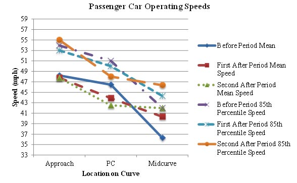
Figure 51. Graph. U.S. Route 219 treatment site A (MM 6.32) operating speeds (PSL = 55 mph).
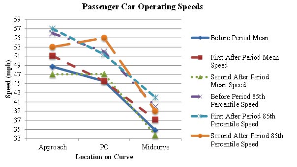
Figure 52. Graph. U.S. Route 219 treatment site B (MM 5.81) operating speeds (PSL=55 mph).
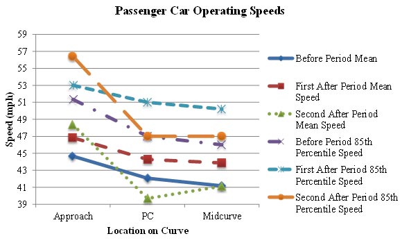
Figure 53. Graph. U.S. Route 219 comparison site operating speeds (PSL = 55 mph).
In summary, the research team compared the mean operating speed for passenger cars and trucks before and at two different time periods after installing the HFST at four treatment and three comparison sites in West Virginia. The mean speeds were compared during the three data- collection time periods at a location on the approach tangent, curve PC location, and the midpoint of the horizontal curve. The analysis included only daytime and unopposed free-flow vehicle mean speeds.
The results of the mean speed analysis indicate that the HFST did not significantly affect vehicle mean operating speeds in a consistent manner across all four treatment sites. Few of the independent sample t-tests showed that the mean passenger car and heavy truck operating speeds differed between the before and first or second after periods at the treatment sites. A multifactor analysis of variance (ANOVA) found that the data collection-time period–treatment site interaction was not statistically significant (F2, 4160 = 0.49, p > 0.05) at the approach speed location, when including observations of free-flow vehicles only and controlling for the presence of vehicles in the opposing lane, time of day, and vehicle type. Similar results were found at the PC (F2, 4160 = 1.51, p > 0.05) and midcurve locations (F2, 4160 = 0.56, p > 0.05).
Change in Mean Operating Speed
The next measure considered in the analysis was the change in speed from the PC to the midpoint of the horizontal curve (hereafter referred to as delta speed). This measure was observed in the before and both after periods at each of the treatment and comparison sites. As discussed previously, researchers used a t-test for independent samples to compare the two after periods with the before period and to compare the two after periods with one another. Table 26 shows the change in speed (delta speed) from the entry of the curve to the midpoint of the curve. The positive value of delta speed indicates that a mean decrease in speed occurred from the PC to the midpoint of the curve. A negative value represents a mean increase in speed between the two locations. As expected, few locations demonstrated a mean increase in speed from the PC to midcurve location.
Table 26. Change in speed from PC to curve midpoint.
| Speed Metric | Delta Speed |
Standard Deviation |
N |
| U.S. Route 219 Treatment 6.32 PCs before | 10.174 |
8.896 |
86 |
| U.S. Route 219 Treatment 6.32 PCs 1st after | 3.536 |
5.629 |
97 |
| U.S. Route 219 Treatment 6.32 PCs 2nd after | 0.544 |
4.913 |
90 |
| U.S. Route 219 Treatment 6.32 trucks before | 9.909 |
9.016 |
11 |
| U.S. Route 219 Treatment 6.32 trucks 1st after | 2.813 |
4.004 |
16 |
| U.S. Route 219 Treatment 6.32 trucks 2nd after | -0.6 |
3.715 |
5 |
| U.S. Route 219 Treatment 5.81 PCs before | 10.747 |
7.923 |
79 |
| U.S. Route 219 Treatment 5.81 PCs 1st after | 8.417 |
7.239 |
103 |
| U.S. Route 219 Treatment 5.81 PCs 2nd after | 13.38 |
6.779 |
71 |
| U.S. Route 219 Treatment 5.81 trucks before | 7 |
7.165 |
13 |
| U.S. Route 219 Treatment 5.81 trucks 1st after | 7.889 |
1.691 |
9 |
| U.S. Route 219 Treatment 5.81 trucks 2nd after | 13 |
2.828 |
2 |
| U.S. Route 219 Comparison PCs before | 0.9 |
4.586 |
50 |
| U.S. Route 219 Comparison PCs 1st after | 0.423 |
5.008 |
71 |
| U.S. Route 219 Comparison PCs 2nd after | -1.439 |
9.859 |
41 |
| U.S. Route 219 Comparison trucks before | 0.429 |
7.231 |
7 |
| U.S. Route 219 Comparison trucks 1st after | 0.286 |
1.976 |
7 |
| U.S. Route 219 Comparison trucks 2nd after | -0.455 |
8.067 |
11 |
| U.S. Route 33 Treatment PCs before | 7.177 |
5.367 |
158 |
| U.S. Route 33 Treatment PCs 1st after | 7.632 |
4.953 |
163 |
| U.S. Route 33 Treatment PCs 2nd after | 11.182 |
7.653 |
143 |
| U.S. Route 33 Treatment trucks before | 5.105 |
3.71 |
19 |
| U.S. Route 33 Treatment trucks 1st after | 1.667 |
6.391 |
24 |
| U.S. Route 33 Treatment trucks 2nd after | 3.429 |
6.25 |
21 |
| U.S. Route 33 Comparison PCs before | 3.178 |
8.494 |
118 |
| U.S. Route 33 Comparison PCs 1st after | 2.902 |
6.393 |
133 |
| U.S. Route 33 Comparison PCs 2nd after | 3.486 |
5.312 |
142 |
| U.S. Route 33 Comparison trucks before | 3.286 |
8.09 |
14 |
| U.S. Route 33 Comparison trucks 1st after | 1.379 |
5.551 |
29 |
| U.S. Route 33 Comparison trucks 2nd after | 2.15 |
2.925 |
20 |
| WV Route 32 Treatment PCs before | 5.689 |
5.856 |
167 |
| WV Route 32 Treatment PCs 1st after | 5.783 |
7.091 |
175 |
| WV Route 32 Treatment PCs 2nd after | 5.216 |
7.072 |
199 |
| WV Route 32 Treatment trucks before | 1.667 |
4.179 |
6 |
| WV Route 32 Treatment trucks 1st after | 8.875 |
3.758 |
8 |
| WV Route 32 Treatment trucks 2nd after | 2.917 |
6.007 |
12 |
| WV Route 32 Comparison PCs before | 2.282 |
7.139 |
124 |
| WV Route 32 Comparison PCs 1st after | 2.357 |
4.548 |
185 |
| WV Route 32 Comparison PCs 2nd after | 2.933 |
4.97 |
240 |
| WV Route 32 Comparison trucks before | 4.429 |
4.117 |
7 |
| WV Route 32 Comparison trucks 1st after | 1.889 |
4.197 |
9 |
| WV Route 32 Comparison trucks 1st after | 2.688 |
5.474 |
16 |
As table 26 shows, there was no statistically significant change in delta speed at any of the comparison locations for either passenger cars or heavy trucks. The only changes that occurred for passenger cars in the first after period were at the U.S. Route 219 treatment sites. In both cases, the delta speed was reduced (more constant speeds from the approach to the midpoint of the curve). Speeds became even more constant between the PC and midcurve in the second after treatment period at the first treatment site (MM 6.32) of U.S. Route 219, with less than a 1-mph change between the PC and curve midpoint. There was also a change at the second treatment site (MM 5.81) in the second after period; however, this change was an increase in delta speed of approximately 2.6 mph from the before period. This increase in delta speed is probably associated with passenger vehicles entering the curve at a higher speed in the second after period relative to the before period, and then realizing they are travelling too fast for the curve. There was also an increase in delta speed at the U.S. 33 treatment site in the second after period. The change was approximately 4 mph relative to the before period.
A statistically significant change was found for heavy trucks at three out of the four treatment sites in the first after period. The delta speed was significantly reduced at two sites (by 7.1 mph and 3.5 mph). One treatment site showed a significant increase in delta speed (7.2 mph) from the before to the first after period; however, it is noted that there were only six heavy vehicles in the before period and eight heavy vehicles in the after period. The very low SD in both cases for this site shows that outliers are not driving these results. However, delta speed was reduced by 6 mph from the first after period to the second after period, and was 1.3 mph greater than in the before period. The site with the 7.1 mph reduction in delta speed in the first after period also had a 3.4 mph reduction from the first after period to the second after period. Delta speed actually became slightly negative at this site, representing an increase in speed from the PC to the curve midpoint.
There is no consistent trend in the difference between passenger car speeds at the PC and curve midpoint from the before to the second after period as a result of the HFST. There was a significant increase in the difference at two treatment sites, but there was also a very significant decrease in the difference at another treatment site. The site (U.S. Route 219 Treatment 6.32) with the decrease in delta speed for passenger cars also had a statistically significant decrease in delta speed for trucks. A multifactor ANOVA found that the treatment site-time period interaction was not statistically significant (F2, 4160 = 0.51, p > 0.05) when including observations of free-flow vehicles only and controlling for the presence of vehicles in the opposing lane, time of day, and vehicle type. This suggests that the HFST did not affect the change in vehicle speeds between the PC and midcurve locations in the current study.
Vehicles Exceeding Posted Speed Limit
Finally, in addition to the t-test, the percentage of vehicles exceeding the PSL and the advisory speed at the treatment and control sites was calculated and compared between data-collection periods. The following describes the results of the data analysis.
Table 27 shows the number of passenger cars and heavy trucks observed to exceed the speed limit at each location of every site in the before and both after periods. A test of proportions was used to determine whether the proportion of speeding vehicles changed at each location of every site from the before to after treatment application. From table 27, there were no visible trends from the before period to after treatment application. In the first after period, there was only a significant change in the number of passenger vehicles exceeding the speed limit at the first treatment site of U.S. Route 219 (MM 6.32), where the proportion of vehicles exceeding the speed limit at the PC was lower relative to the before period. Four vehicles exceeded the speed limit in the before period, and no vehicles exceeded the speed limit in the first and second after periods. This change was also significant in the second after period. There was one additional site in the second after period that had a significant reduction in the number of vehicles exceeding the speed limit. At the WV Route 32 treatment site, the proportion was reduced from 0.50 to 0.39 at the approach point. There were also a few locations where there was a significant difference between the two after periods, but not the before period, which resulted from a slight reduction in the first after period that was not statistically significant. The only statistically significant change at the curve midpoint was at the WV Route 32 comparison site, where the proportion of trucks exceeding the speed limit significantly increased in the first after period, but then the proportion decreased in the second after period and was no longer significant. This result is noteworthy, however, because the U.S. Route 219 and U.S. Route 33 sites had such restrictive geometry that few vehicles traveled in excess of the PSL.
Table 27. Number of vehicles exceeding the PSL by site.
Data-Collection Location and Time Period |
Speed Observation Site |
|||||||
U.S. Route 219 |
U.S. Route 33 |
WV Route 32 |
||||||
Treat. A (MM6.32) |
Treat. B (MM5.81) |
Comp. |
Treat. |
Comp. |
Treat. |
Comp. |
||
Approach passenger cars |
Before |
6(7%) |
15(19%) |
3(6%) |
15(9%) |
1(1%) |
83(50%) |
82(60%) |
1st After |
10(10%) |
23(22%) |
5(7%) |
12(7%) |
3(2%) |
75(43%) |
121(65%) |
|
2nd After |
12(13%) |
8(11%) |
1(9%) |
21(15%) |
3(2%) |
77(39%) |
5(71%) |
|
Approach trucks |
Before |
1(9%) |
2(15%) |
1(14%) |
0(0%) |
0(0%) |
4(67%) |
5(71%) |
1st After |
1(6%) |
1(11%) |
0(0%) |
0(0%) |
0(0%) |
5(63%) |
5(56%) |
|
2nd After |
0(0%) |
0(0%) |
2(50%) |
0(0%) |
0(0%) |
4(33%) |
5(31%) |
|
PC passenger cars |
Before |
4(5%) |
5(6%) |
0(0%) |
0(0%) |
>
1(1%) |
63(38%) |
60(48%) |
1st After |
0(0%) |
2(2%) |
3(4%) |
3(2%) |
0(0%) |
52(30%) |
81(44%) |
|
2nd After |
0(0%) |
8(11%) |
3(7%) |
2(1%) |
0(0%) |
62(31%) |
125(52%) |
|
PC trucks |
Before |
1(9%) |
0(0%) |
0(0%) |
0(0%) |
0(0%) |
2(33%) |
1(14%) |
1st After |
0(0%) |
0(0%) |
0(0%) |
0(0%) |
0(0%) |
2(25%) |
3(33%) |
|
2nd After |
0(0%) |
0(0%) |
4(36%) |
0(0%) |
0(0%) |
3(25%) |
5(31%) |
|
Midcurve passenger cars |
Before |
1(1%) |
1(1%) |
0(0%) |
0(0%) |
2(2%) |
12(7%) |
45(36%) |
1st After |
1(1%) |
2(2%) |
0(0%) |
0(0%) |
0(0%) |
5(3%) |
48(26%) |
|
2nd After |
1(1%) |
2(2%) |
0(0%) |
0(0%) |
0(0%) |
18(9%) |
74(31%) |
|
Midcurve trucks |
Before |
0(0%) |
0(0%) |
0(0%) |
0(0%) |
0(0%) |
0(0%) |
0(0%) |
1st After |
0(0%) |
0(0%) |
0(0%) |
0(0%) |
0(0%) |
0(0%) |
3(33%) |
|
2nd After |
0(0%) |
0(0%) |
0(0%) |
0(0%) |
0(0%) |
0(0%) |
1(6%) |
|
Number of passenger cars |
Before |
86 |
79 |
50 |
158 |
118 |
167 |
124 |
1st After |
97 |
103 |
71 |
163 |
133 |
175 |
185 |
|
2nd After |
90 |
71 |
11/41a |
143 |
142 |
199 |
240 |
|
Number of trucks |
Before |
11 |
13 |
7 |
19 |
14 |
6 |
7 |
1st After |
16 |
9 |
7 |
24 |
29 |
8 |
9 |
|
2nd After |
5 |
2 |
4/11b |
21 |
20 |
12 |
16 |
|
aEleven observations at the approach point and 41 observations at the PC and midcurve.
bFour observations at the approach point and 11 observations at the PC and midcurve.
Bold indicates significance at the 95-percent confidence level (α =0.05) between the 1st/2nd after period and before period.
Italics indicates significance at the 95-percent confidence level (α=0.05) between the 1st and 2nd after periods.
Treat. = Treatment
MM = Mile
Marker
Comp. = Comparison
PC = Point of Curvature
Table 28 shows the number of vehicles exceeding the advisory speed at the midpoint of the curve for each study site. The research team considered only the midpoint location because the advisory speed is for the horizontal curve, and the approach and PC locations are not within the curve. No significant changes were observed at the comparison sites from the before to the first after period. The proportion of passenger cars exceeding the advisory speed was significantly higher at the U.S. Route 219 treatment A (MM 6.32) site, but there was no change at any other site in the first after period. This increase continued into the second after period, where all but one vehicle exceeded the advisory speed. The proportion of heavy trucks exceeding the advisory speed was significantly lower at the WV Route 32 site in the first after period, but there was no change at any other site. This reduction did not continue into the second after period and the proportion of trucks exceeding the advisory speed was 100 percent, which is the same as in the before period. In the second after period at the U.S. Route 219 treatment B (MM 5.81) site, there was a significant decrease in the proportion of vehicles exceeding the advisory speed when compared with the before and first after periods. At this same site, the proportion of trucks exceeding the advisory speed was also significantly reduced when compared with the before and first after periods. There was also a significant reduction at the U.S. Route 219 comparison site between the first after period and second after period. This reduction was less significant than at the treatment B site. The proportion of vehicles decreased by 0.08 compared with the before period at the comparison site and 0.19 at the treatment site B. The proportion of passenger cars exceeding the advisory speed increased at one treatment site, decreased at another treatment site, and remained the same at the other two. These results indicate there might be a slight reduction in the number of trucks exceeding the advisory speed, but there does not appear to be a strong effect on the number of passenger vehicles exceeding the advisory speed at the HFST locations.
Table 28. Number of vehicles exceeding the advisory speed by site.
Data-Collection Location and Time Period |
Speed Observation Site |
|||||||
U.S. Route 219 |
U.S. Route 33 |
WV Route 32 |
||||||
Treat. A (MM6.32) |
Treat. B (MM5.81) |
Comp. |
Treat. |
Comp. |
Treat. |
Comp. |
||
Midcurve passenger cars |
Before |
74(86%) |
75(95%) |
49(98%) |
148(94%) |
111(94%) |
154(92%) |
80(65%) |
1st After |
94(97%) |
100(97%) |
70(99%) |
148(91%) |
124(93%) |
159(91%) |
155(65%) |
|
2nd After |
89(99%) |
54(76%) |
37(90%) |
129(90%) |
134(94%) |
177(89%) |
155(65%) |
|
Midcurve trucks |
Before |
8(73%) |
13(100%) |
7(100%) |
13(68%) |
12(86%) |
6(100%) |
3(43%) |
1st After |
15(94%) |
9(100%) |
5(71%) |
16(67%) |
22(76%) |
5(50%) |
4(44%) |
|
2nd After |
4(80%) |
1(50%) |
11(100%) |
9(43%) |
19(95%) |
12(100%) |
6(38%) |
|
Number of passenger cars |
Before |
86 |
79 |
50 |
158 |
118 |
167 |
124 |
1st After |
97 |
103 |
71 |
163 |
133 |
175 |
185 |
|
2nd After |
90 |
71 |
41 |
143 |
142 |
199 |
240 |
|
Number of trucks |
Before |
11 |
13 |
7 |
19 |
14 |
6 |
7 |
1st After |
16 |
9 |
7 |
24 |
29 |
8 |
9 |
|
2nd After |
5 |
2 |
11 |
21 |
20 |
12 |
16 |
|
Bold indicates significance at the 95-percent confidence level (α =0.05) between the 1st/2nd after period and before period.
Italics indicates significance at the 95-percent confidence level (α=0.05) between the 1st and 2nd after periods.
Treat. = Treatment
MM = Mile
Marker
Comp. = Comparison
PC = Point of Curvature
Speed variance was the final speed performance metric considered in the current study. A two- sided F-test was used to compare the variance of vehicle operating speed in the before and after periods for passenger cars and heavy trucks.
Table 29 shows that the only change that occurred for the U.S. Route 219 comparison site in the first after period was at the PC for passenger cars. There was an approximate 1.5-mph increase in speed deviation at this location. Taking this change into account, the speed deviation was found to decrease at the PC locations for both treatment sites. There was also a significant decrease at the approach location for treatment site B for both passenger cars and heavy trucks, as well as at the midpoint of the curve at treatment site A for passenger cars. For the U.S. Route 219 comparison site, there was an increase in speed deviation at the PC and curve midpoint in the second after period compared with the before period. There was an approximate 6.4-mph increase in speed deviation at the PC and an approximate 1.5-mph increase at the curve midpoint. Taking these changes into account, there was a decrease in speed deviation at the PC and curve midpoint for both treatment sites. There was only a significant decrease between the first and second after period for trucks at the midpoint of the curve of the comparison site. However, there was no change between the before and second after period. There was also no change in speed deviation at any data-collection point for trucks at the two treatment sites.
When comparing the first after period with the before period for U.S. Route 33 comparison site, the speed deviation decreased by 1.3 mph at the PC for passenger cars and increased by approximately 3.5 mph at the approach and PC for heavy trucks. Taking these trends into account, a significant increase in speed deviation occurred at the approach and PC for passenger cars, while a significant decrease occurred at the midpoint of the horizontal curve. For heavy trucks, a significant increase occurred only at the PC (approximately 2.7 mph). At the comparison site, the speed deviation decreased by approximately 1.3 mph at the curve midpoint for passenger cars. There was also a statistically significant increase at the approach for passenger cars, but this was only between the first and second after periods. Taking these trends into account, a significant increase in speed deviation occurred at the curve midpoint for passenger cars in the second after period. At the comparison site, there was no statistically significant change in speed deviation between the before and second after period for trucks. There was a statistically significant decrease at the approach and PC location for trucks between the first and second after periods. The speed deviation increased by approximately 3.9 mph at the PC for trucks from the before to second after period at the treatment site.
For WV Route 32, there were statistically significant decreases at the PC and the midpoint of the curve for passenger cars and significant increases at the approach and PC for heavy trucks at the comparison site in the first after period. Taking these differences into account resulted in statistically significant increases in speed deviation at the PC and midpoint for passenger cars, and significant decreases for heavy trucks at the approach and PC for heavy trucks at the treatment site. In the second after period, there was a significant increase in speed deviation at the PC and a significant decrease at the curve midpoint for the comparison site for passenger cars. Taking these differences into account, there was a significant increase in speed deviation at the approach and curve midpoint of the treatment site for passenger cars in the second after period. There was also a significant increase in speed deviation at the approach and PC for trucks at the comparison site. Taking these differences into account, there was a significant decrease in speed deviation at the approach and PC for the treatment site for trucks in the second after period.
There was no consistent trend in the effects of the HFST on the speed deviation of passenger cars. The effects of the HFST on the speed deviation were considered for the PC and curve midpoint locations because the surface was applied starting at the PC, or just before it, and it was assumed that the surface would have no effect on the speed deviation at the approach data- collection location. In the first after period, the speed deviation increased at the PC for two sites, but the speed deviation also decreased at two other sites. In the second after period, the speed deviation decreased at the PC for two sites. In the first after period, the speed deviation increased at the curve midpoint at one site, but the speed deviation decreased at another site. In the second after period, the speed deviation increased at the curve midpoint for two sites, but the speed deviation also decreased at two sites. For trucks, the speed deviation decreased at the PC at one site in both after periods, and it also decreased at one site in both after periods. There was no change in speed deviation at the curve midpoint for trucks at any site.
Table 29. Change in standard deviation of speed.
| Speed Metric | Approach SD |
PC SD |
Mid SD |
N |
| U.S. Route 219 Treatment 6.32 PCs before | 6.282 |
6.135 |
7.221 |
86 |
| U.S. Route 219 Treatment 6.32 PCs 1st after | 6.219 |
5.251 |
5.433 |
97 |
| U.S. Route 219 Treatment 6.32 PCs 2nd after | 7.204 |
5.637 |
4.72 |
90 |
| U.S. Route 219 Treatment 6.32 trucks before | 5.971 |
6.44 |
4.698 |
11 |
| U.S. Route 219 Treatment 6.32 trucks 1st after | 5.118 |
6.017 |
5.092 |
16 |
| U.S. Route 219 Treatment 6.32 trucks 2nd after | 7.517 |
5.413 |
4.919 |
5 |
| U.S. Route 219 Treatment 5.81 PCs before | 8.825 |
7.412 |
6.728 |
79 |
| U.S. Route 219 Treatment 5.81 PCs 1st after | 5.788 |
5.489 |
6.463 |
103 |
| U.S. Route 219 Treatment 5.81 PCs 2nd after | 7.617 |
7.484 |
5.197 |
71 |
| U.S. Route 219 Treatment 5.81 trucks before | 8.19 |
5.964 |
3.728 |
13 |
| U.S. Route 219 Treatment 5.81 trucks 1st after | 3.395 |
4.444 |
4.466 |
9 |
| U.S. Route 219 Treatment 5.81 trucks 2nd after | 2.828 |
7.778 |
4.95 |
2 |
| U.S. Route 219 Comparison PCs before | 6.317 |
4.867 |
4.354 |
50 |
| U.S. Route 219 Comparison PCs 1st after | 5.967 |
6.388 |
5.354 |
71 |
| U.S. Route 219 Comparison PCs 2nd after | 7.915 |
11.257 |
5.802 |
11/41a |
| 11/41U.S. Route 219 Comparison trucks before | 8.08 |
5.908 |
4.10 |
7 |
| U.S. Route 219 Comparison trucks 1st after | 10.04 |
8.591 |
7.925 |
7 |
| U.S. Route 219 Comparison trucks 2nd after | 8.164 |
6.439 |
3.33 |
4/11b |
| 4/11U.S. Route 33 Treatment PCs before | 6.538 |
5.346 |
4.571 |
158 |
| U.S. Route 33 Treatment PCs 1st after | 7.512 |
5.771 |
3.791 |
163 |
| U.S. Route 33 Treatment PCs 2nd after | 7.723 |
7.199 |
5.024 |
143 |
| U.S. Route 33 Treatment trucks before | 7.762 |
3.7 |
4.188 |
19 |
| U.S. Route 33 Treatment trucks 1st after | 11.329 |
8.855 |
4.967 |
24 |
| U.S. Route 33 Treatment trucks 2nd after | 9.049 |
7.593 |
5.661 |
21 |
| U.S. Route 33 Comparison PCs before | 5.812 |
6.318 |
6.786 |
118 |
| U.S. Route 33 Comparison PCs 1st after | 5.372 |
5.055 |
6.086 |
133 |
| U.S. Route 33 Comparison PCs 2nd after | 6.462 |
5.812 |
5.445 |
142 |
| U.S. Route 33 Comparison trucks before | 5.409 |
5.045 |
5.698 |
14 |
| U.S. Route 33 Comparison trucks 1st after | 8.918 |
8.461 |
7.41 |
29 |
| U.S. Route 33 Comparison trucks 2nd after | 5.569 |
4.921 |
5.781 |
20 |
| WV Route 32 Treatment PCs before | 7.3 |
6.283 |
5.639 |
167 |
| WV Route 32 Treatment PCs 1st after | 7.959 |
7.343 |
5.126 |
175 |
| WV Route 32 Treatment PCs 2nd after | 8.447 |
6.645 |
7.212 |
199 |
| WV Route 32 Treatment trucks before | 3.987 |
5.089 |
4.622 |
6 |
| WV Route 32 Treatment trucks 1st after | 3.227 |
5.855 |
4.658 |
8 |
| WV Route 32 Treatment trucks 2nd after | 6.443 |
5.384 |
3.477 |
12 |
| WV Route 32 Comparison PCs before | 6.04 |
6.046 |
7.617 |
124 |
| WV Route 32 Comparison PCs 1st after | 5.317 |
5.057 |
5.587 |
185 |
| WV Route 32 Comparison PCs 2nd after | 6.315 |
6.923 |
6.06 |
240 |
| WV Route 32 Comparison trucks before | 2.992 |
2.734 |
3.823 |
7 |
| WV Route 32 Comparison trucks 1st after | 8.023 |
5.94 |
5.148 |
9 |
| WV Route 32 Comparison trucks 2nd after | 6.811 |
6.708 |
3.373 |
16 |
aEleven observations at the approach point and 41 observations at the PC and midcurve.
bFour observations at the approach point and 11 observations at the PC and midcurve.
Bold indicates
significance at the 95-percent confidence level (α =0.05) between the 1st and 2nd after periods relative to the
before period.
Italics indicates significance at 95-percent confidence level (α =0.05) between the 1st and 2nd after
periods.
SD = Standard Deviation
PC = Point of Curvature
N= Number of Observations
Along with speed metrics, the research team observed encroachment and braking vehicles; table 30 shows these data. The data collection and analysis methods were described earlier in this report.
Table 30 shows the braking and encroachment data for the comparison and treatment sites. There was no statistically significant change in the before or first after period—for any braking or encroachment measure—at treatment site A along U.S. Route 219. At treatment site B along U.S. Route 219, there was a statistically significant reduction in the proportion of vehicles entering the curve that encroached onto the shoulder and those vehicles entering the curve that encroached over the centerline, when comparing the before with the first after period. However, these reductions did not continue into the second after period, and there were no statistically significant change in the second after period relative to the before period. At the U.S. Route 219 comparison site, there was a reduction in the proportion of vehicles entering the curve that encroached onto the shoulder in the second after period. There was also a reduction in the proportion of vehicles entering the curve that braked inside the curve and a reduction in the proportion of vehicles exiting the curve that encroached beyond centerline, when comparing the before with the first after period. However, these reductions did not continue into the second after period, and there were no reductions in the second after period relative to the before period.
There was a reduction in the proportion of vehicles entering the curve that encroached on the centerline in the first after period at the U.S. Route 33 treatment site, but there was no reduction in the second after period. At both the U.S. Route 33 treatment and comparison sites, there was a reduction in the proportion of vehicles entering the curve that braked before the curve in the first after period, but there was no reduction in the second after period, relative to the before period. At the treatment site, there was a statistically significant increase in the proportion of vehicles exiting the curve that encroached onto the shoulder, in both after periods. There was also a significant reduction in the proportion of vehicles exiting the curve that crossed the centerline between the two lanes in the first after period, but once again, this reduction did not continue into the second after period.
At the WV Route 32 treatment site, there was an increase in the proportion of vehicles entering the curve that braked inside the curve in the first after period, but there was no change in the second after period relative to the before period. At the WV Route 32 treatment site, the camera was placed so it could see before the curve in the second after period, where it could not in the before and first after period. As a result, a statistical analysis of the braking before/within the curve for this site was not conducted in the second after period. There was also a reduction in the proportion of vehicles entering the curve that encroached onto the shoulder in the second after period at the treatment site. This significant reduction becomes more significant after accounting for the comparison site because there was an increase in the proportion of vehicles entering the curve that encroached onto the shoulder. Finally, at the WV Route 32 comparison site, there was a reduction in the proportion of vehicles entering the curve that braked before the curve in the first after period, but there was an increase in the second after period.
There was no significant change in the braking and encroachment data that lasted throughout the treatment period except for an increase in the proportion of vehicles exiting the curve that encroached onto the shoulder at the U.S. Route 33 treatment site and also a decrease in the proportion of vehicles entering the curve that encroached onto the shoulder at the WV Route 32 treatment site. These results show the HFST does not have a consistent effect on the braking and encroachment behavior of vehicles.
Table 30. Number of encroachments and braking vehicles by site.
Data-Collection Location and Time Period |
Speed Observation Site |
|||||||
U.S. Route 219 |
U.S. Route 33 |
WV Route 32 |
||||||
Treat. A (MM6.32) |
Treat. B (MM5.81) |
Comp. |
Treat. |
Comp. |
Treat. |
Comp. |
||
Total Entering |
Before |
77 |
61 |
49 |
122 |
89 |
127 |
110 |
1st After |
91 |
74 |
111 |
104 |
80 |
102 |
122 |
|
2nd After |
89 |
77 |
39 |
103 |
81 |
74 |
68 |
|
Entering Shoulder |
Before |
2(3%) |
10(16%) |
8(16%) |
6(5%) |
4(4%) |
17(13%) |
2(2%) |
1st After |
3(3%) |
0(0%) |
12(11%) |
4(4%) |
4(5%) |
11(11%) |
3(2%) |
|
2nd After |
8(9%) |
5(6%) |
1(3%) |
11(11%) |
7(9%) |
1(1%) |
8(12%) |
|
Entering Centerline |
Before |
0(0%) |
10(16%) |
0(0%) |
15(12%) |
10(11%) |
0(0%) |
0(0%) |
1st After |
1(1%) |
5(5%) |
0(0%) |
5(5%) |
8(10%) |
1(1%) |
0(0%) |
|
2nd After |
3 |
10 |
0(0%) |
8(8%) |
4(5%) |
3(4%) |
0(0%) |
|
Entering Brake Before |
Before |
56(73%) |
31(51%) |
N/A |
115(94%) |
85(96%) |
N/A |
15(14%) |
1st After |
75(82%) |
43(58%) |
N/A |
87(84%) |
62(78%) |
N/A |
6(5%) |
|
2nd After |
70(79%) |
50(65%) |
N/A |
96(93%) |
79(98%) |
16(22%) |
18(26%) |
|
Entering Brake Inside |
Before |
12(16%) |
20(33%) |
47(96%) |
3(2%) |
2(2%) |
35(28%) |
10(9%) |
1st After |
6(7%) |
27(36%) |
83(75%) |
4(4%) |
10(13%) |
53(52%) |
17(14%) |
|
2nd After |
7(8%) |
23(30%) |
38(97%) |
5(5%) |
1(1%) |
23(31%) |
6(9%) |
|
Total Exiting |
Before |
92 |
61 |
60 |
130 |
92 |
132 |
129 |
1st After |
69 |
62 |
78 |
124 |
93 |
96 |
97 |
|
2nd After |
90 |
71 |
33 |
94 |
100 |
88 |
76 |
|
Exiting Shoulder |
Before |
3(3%) |
2(3%) |
3(5%) |
1(1%) |
12(13%) |
6(5%) |
0(0%) |
1st After |
3(4%) |
1(2%) |
1(1%) |
9(7%) |
5(5%) |
5(5%) |
0(0%) |
|
2nd After |
2(2%) |
2(3%) |
0(0%) |
18(19%) |
9(9%) |
2(2%) |
1(1%) |
|
Exiting Centerline |
Before |
6(7%) |
12(20%) |
20(33%) |
2(2%)[48](37%) |
5(5%) |
12(9%) |
6(5%) |
1st After |
3(4%) |
5(8%) |
11(14%) |
0(0%)[20](16%) |
3(3%) |
7(7%) |
4(4%) |
|
2nd After |
10(1%) |
16(23%) |
12(36%) |
0(0%)[24](26%) |
4(4%) |
7(8%) |
3(4%) |
|
Bold indicates significance at the 95-percent confidence level (α =0.05) between the 1st/2nd after period and before period.
Italics indicates significance at the 95-percent confidence level (α =0.05) between the 1st and 2nd after periods.
Brackets indicate encroachment on broken line for U.S. 33 treatment site in uphill (exiting) direction
Treat. = Treatment
MM = Mile Marker
Comp. = Comparison
The research team used the DF tester and CT meter to evaluate the skid resistance of the treatment and comparison site locations. The data collection and analysis methods were described earlier in this report. Table 31 through table 33 show the before, first after, and second after period friction data, respectively. The values reported in each table correspond to the SN at 40 mph. As table 31 shows, the minimum friction value observed in the before period was 0.26, and the maximum friction value was 0.46. As noted above, the research team observed friction values across the curve approach to determine whether a trend existed. As the data show, there was no discernible trend across the approaches (where deceleration occurs). The data do show that there is not a consistent level of friction across each approach, but each location varies with respect to its adjacent location differently at each site. As for the horizontal curve, there is a large amount of variability in pavement friction within each horizontal curve in the before period. At the WV Route 32 and U.S. Route 33 sites, the minimum friction level occurred at the three-quarter point of the horizontal curve; however, this was not the case at the U.S. Route 219 sites. At the U.S. Route 219 sites, the minimum friction level occurred at the one-quarter point or the midpoint of the horizontal curve. Otherwise, there are no apparent patterns within the horizontal curves with regard to friction supply.
Table 31. SN65 friction data from the before period.
| Site | 300 ft |
200 ft |
100 ft |
PC |
1/4 |
Midcurve |
3/4 |
PT |
| WV Route 32 Treatment | 0.41 |
0.46 |
0.40 |
0.39 |
0.32 |
0.38 |
0.31 |
0.32 |
| WV Route 32 Comparison | 0.38 |
0.41 |
0.40 |
0.36 |
0.36 |
0.36 |
0.28 |
0.42 |
| U.S. Route 33 Treatment | 0.33 |
0.34 |
0.34 |
0.40 |
0.33 |
0.32 |
0.32 |
0.36 |
| U.S. Route 33 Comparison | N/A |
N/A |
0.31 |
0.34 |
0.28 |
0.28 |
0.26 |
0.29 |
| U.S. Route 219 Treatment MM 6.32 | 0.38 |
0.37 |
0.36 |
0.40 |
0.36 |
0.38 |
0.37 |
0.40 |
| U.S. Route 219 Treatment MM 5.81 | 0.38 |
0.40 |
0.40 |
0.41 |
0.40 |
0.35 |
0.44 |
0.40 |
| U.S. Route 219 Comparison | N/A |
N/A |
0.31 |
0.32 |
0.29 |
0.30 |
0.33 |
0.32 |
MM = Mile Marker
PT = Point of Tangent
N/A = Not Applicable
Table 32 presents the friction data from the immediate after-application period. The HFST was only applied within the horizontal curves (from the PC to the PT) at each treatment site. This means that the approach data at every site and all data at the comparison sites should be comparable. The treatment surface was applied from the PC to the PT for each of the treatment curves. For the WV Route 32 treatment site, it is readily apparent that the treatment application was not uniform—the observed friction decreased from the PC to the PT. At the other three sites, the application appeared to provide the greatest observed friction at the PC and PT; the friction across the middle of the curve was lower than at the ends of the curve.
Table 32. SN65 friction data from the immediate after period.
| Site | 300 ft |
200 ft |
100 ft |
PC |
1/4 |
Midcurve |
3/4 |
PT |
| WV Route 32 Treatment | 0.31 |
0.42 |
0.43 |
0.72 |
0.67 |
0.66 |
0.62 |
0.57 |
| WV Route 32 Comparison | 0.32 |
0.32 |
0.37 |
0.35 |
0.33 |
0.33 |
0.35 |
0.38 |
| U.S. Route 33 Treatment | 0.36 |
0.32 |
0.38 |
0.62 |
0.60 |
0.51 |
0.56 |
0.58 |
| U.S. Route 33 Comparison | N/A |
N/A |
0.25 |
0.27 |
0.26 |
0.29 |
0.26 |
0.30 |
| U.S. Route 219 Treatment MM 6.32 | 0.35 |
0.32 |
0.29 |
0.69 |
0.56 |
0.56 |
0.58 |
0.60 |
| U.S. Route 219 Treatment MM 5.81 | 0.37 |
0.38 |
0.34 |
0.65 |
0.61 |
0.62 |
0.60 |
0.66 |
| U.S. Route 219 Comparison | N/A |
N/A |
0.30 |
0.31 |
0.26 |
0.29 |
0.27 |
0.34 |
MM = Mile
Marke r
PT = Point of Tangent
N/A = Not
Applicable
Table 33 shows the friction data from the second after period. As mentioned in the immediate after period at WV Route 32, the observed friction decreased from the PC to PT, with the exception that the observed friction at the PT was almost as high as that at the PC location. The friction levels within the horizontal curve decreased between 0.12 and 0.15 at the WV Route 32 treatment site from the immediate after period to the second after period, with the exception of the PT location, which increased by 0.1. As mentioned in the immediate after period discussion, it is apparent that the treatment was not uniform throughout the curve. The coefficient of friction decreased between 0.10 and 0.15 at the U.S. Route 33 treatment site from the immediate after period to the second after period. The coefficient of friction values at the U.S. Route 219 treatment sites did not change as much between the two after periods as they did at the U.S. Route 33 and WV Route 32 treatment sites.
Table 33. SN65 friction data from the second after period.
| Site | 300 ft |
200 ft |
100 ft |
PC |
1/4 |
Midcurve |
3/4 |
PT |
| WV Route 32 Treatment | 0.36 |
0.38 |
0.36 |
0.59 |
0.55 |
0.51 |
0.50 |
0.58 |
| WV Route 32 Comparison | 0.43 |
0.36 |
0.35 |
0.37 |
0.29 |
0.28 |
0.30 |
0.35 |
| U.S. Route 33 Treatment | 0.32 |
0.34 |
0.34 |
0.51 |
0.46 |
0.38 |
0.46 |
0.43 |
| U.S. Route 33 Comparison | N/A |
N/A |
0.34 |
0.29 |
0.29 |
0.29 |
0.29 |
0.30 |
| U.S. Route 219 Treatment MM 6.32 | 0.33 |
0.36 |
0.34 |
0.59 |
0.58 |
0.59 |
0.61 |
0.61 |
| U.S. Route 219 Treatment MM 5.81 | 0.39 |
0.40 |
0.43 |
0.61 |
0.55 |
0.51 |
0.59 |
0.59 |
| U.S. Route 219 Comparison | N/A |
N/A |
0.33 |
0.37 |
0.29 |
0.32 |
0.36 |
0.36 |
MM = Mile
Marker
PT = Point of Tangent
N/A = Not
Applicable
Table 34 presents the before and after friction data for the treatment site approaches and curves, and also presents the data for the comparison sites. The research team conducted a t-test to compare the before and both after periods of friction data at each site. The test was statistically significant (p-value < 0.05) at each of the four treatment curves in the first after period relative to the before period. The friction level increased significantly from the before to the after period at the treatment sites, ranging from an increase of 0.21 to 0.30 in the SN65 value. At all four treatment sites, the second after period produced friction levels that were statistically higher than the before period, indicating that the higher friction levels produced by the treatment were maintained for at least one year. Only two sites had friction values that were not significantly different from the before to the after period. The first was the approach to the WV Route 32 treatment site and the second was the U.S. 219 comparison site. This means that for the rest of the treatment approaches and comparison sites (none of which were treated with a high-friction surface), the before and after friction cannot be treated as the same value. The differences were marginal, as can be noted from table 34, but may indicate differences resulting from weather conditions or some other confounding factor from the before period (in May) to the after period (in August). Because of these findings, the before and after friction data at the comparison and non-treatment sites were considered independently in the margin of safety analysis.
Table 34. Before and after friction data for comparison.
| Location | Mean |
Standard Deviation |
N |
t-stat |
| WV Route 32 Treatment Approach before | 0.424 |
0.032 |
6 |
N/A |
| WV Route 32 Treatment Approach 1st after | 0.386 |
0.068 |
6 |
-1.24 |
| WV Route 32 Treatment Approach 2nd after | 0.365 |
0.015 |
6 |
-4.14 |
| WV Route 32 Treatment Curve before | 0.347 |
0.037 |
10 |
N/A |
| WV Route 32 Treatment Curve 1st after | 0.646 |
0.057 |
10 |
13.90 |
| WV Route 32 Treatment Curve 2nd after | 0.543 |
0.040 |
10 |
11.35 |
| WV Route 32 Comparison Site before | 0.370 |
0.044 |
16 |
N/A |
| WV Route 32 Comparison Site 1st after | 0.344 |
0.026 |
16 |
-2.04 |
| WV Route 32 Comparison Site 2nd after | 0.341 |
0.050 |
16 |
-1.76 |
| U.S. Route 33 Treatment Approach before | 0.340 |
0.012 |
6 |
N/A |
| U.S. Route 33 Treatment Approach 1st after | 0.369 |
0.017 |
6 |
3.40 |
| U.S. Route 33 Treatment Approach 2nd after | 0.336 |
0.010 |
6 |
-0.56 |
| U.S. Route 33 Treatment Curve before | 0.347 |
0.037 |
10 |
N/A |
| U.S. Route 33 Treatment Curve 1st after | 0.576 |
0.043 |
10 |
12.74 |
| U.S. Route 33 Treatment Curve 2nd after | 0.447 |
0.048 |
10 |
5.23 |
| U.S. Route 33 Comparison Site before | 0.293 |
0.027 |
12 |
N/A |
| U.S. Route 33 Comparison Site 1st after | 0.276 |
0.020 |
12 |
-1.75 |
| U.S. Route 33 Comparison Site 2nd after | 0.301 |
0.020 |
12 |
0.86 |
| U.S. Route 219 Treatment 6.32 Approach before | 0.372 |
0.018 |
6 |
N/A |
| U.S. Route 219 Treatment 6.32 Approach 1st after | 0.318 |
0.029 |
6 |
-3.87 |
| U.S. Route 219 Treatment 6.32 Approach 2nd after | 0.343 |
0.012 |
6 |
-3.34 |
| U.S. Route 219 Treatment 6.32 Curve before | 0.381 |
0.030 |
10 |
N/A |
| U.S. Route 219 Treatment 6.32 Curve 1st after | 0.599 |
0.053 |
10 |
11.32 |
| U.S. Route 219 Treatment 6.32 Curve 2nd after | 0.596 |
0.013 |
10 |
21.12 |
| U.S. Route 219 Treatment 5.81 Approach before | 0.394 |
0.017 |
6 |
N/A |
| U.S. Route 219 Treatment 5.81 Approach 1st after | 0.363 |
0.032 |
6 |
-2.09 |
| U.S. Route 219 Treatment 5.81 Approach 2nd after | 0.406 |
0.021 |
6 |
1.11 |
| U.S. Route 219 Treatment 5.81 Curve before | 0.402 |
0.030 |
10 |
N/A |
| U.S. Route 219 Treatment 5.81 Curve 1st after | 0.631 |
0.028 |
10 |
17.62 |
| U.S. Route 219 Treatment 5.81 Curve 2nd after | 0.570 |
0.040 |
10 |
10.63 |
| U.S. Route 219 Comparison Site before | 0.312 |
0.013 |
12 |
N/A |
| U.S. Route 219 Comparison Site 1st after | 0.296 |
0.030 |
12 |
-1.70 |
| U.S. Route 219 Comparison Site 2nd after | 0.338 |
0.031 |
12 |
2.70 |
Bold indicates
that the difference between the after and before period was statistically significant with a
95-percent confidence.
N = Number of Observations
N/A = Not
Applicable
As table 34 shows, the friction levels decreased throughout the horizontal curves at three treatment sites and remained the same, from the first to second after period, at these same sites. The decreases ranged from 0.061 to 0.129. However, the coefficients of friction were all significantly higher in the second after period than in the before period. t-statistics ranged from 5.23 to 21.12. Friction levels at the comparison sites actually increased slightly at two sites and remained the same at the other site.
The friction data shown in table 35, table 36, and table 37 are longitudinal friction values for the sites. For the margin of safety analysis, the research team estimated the available side (lateral) friction. Lamm et al. has shown that available side (lateral) friction is approximately 92.5 percent of the available longitudinal friction.(74) The authors showed that a multiplier of 0.925 can be used to determine available side (lateral) friction from available longitudinal friction. Table 35, table 36, and table 37show that using this scaling factor, the estimated available side friction (at 40 mph) for the before and both after periods, respectively.
Table 35. SN65 estimated available side friction before treatment application.
| Site | 300 ft |
200 ft |
100 ft |
PC |
1/4 |
Midcurve |
3/4 |
PT |
| WV Route 32 Treatment | 0.38 |
0.43 |
0.37 |
0.36 |
0.30 |
0.35 |
0.29 |
0.30 |
| WV Route 32 Comparison | 0.35 |
0.38 |
0.37 |
0.33 |
0.33 |
0.33 |
0.26 |
0.39 |
| U.S. Route 33 Treatment | 0.31 |
0.31 |
0.31 |
0.37 |
0.31 |
0.30 |
0.30 |
0.33 |
| U.S. Route 33 Comparison | N/A |
N/A |
0.29 |
0.31 |
0.26 |
0.26 |
0.24 |
0.27 |
| U.S. Route 219 Treatment MM 6.32 | 0.35 |
0.34 |
0.33 |
0.37 |
0.33 |
0.35 |
0.34 |
0.37 |
| U.S. Route 219 Treatment MM 5.81 | 0.35 |
0.37 |
0.37 |
0.38 |
0.37 |
0.32 |
0.41 |
0.37 |
| U.S. Route 219 Comparison | N/A |
N/A |
0.29 |
0.30 |
0.27 |
0.28 |
0.31 |
0.30 |
MM = Mile
Marker
PC = Point of Curve
PT = Point of Tangent
N/A = Not
Applicable
Table 36. SN65 Estimated available side friction first after treatment application.
| Site | 300 ft |
200 ft |
100 ft |
PC |
1/4 |
Midcurve |
3/4 |
PT |
| WV Route 32 Treatment | 0.29 |
0.39 |
0.40 |
0.67 |
0.62 |
0.61 |
0.57 |
0.53 |
| WV Route 32 Comparison | 0.30 |
0.30 |
0.34 |
0.32 |
0.31 |
0.31 |
0.32 |
0.35 |
| U.S. Route 33 Treatment | 0.33 |
0.30 |
0.35 |
0.57 |
0.56 |
0.47 |
0.52 |
0.54 |
| U.S. Route 33 Comparison | N/A |
N/A |
0.23 |
0.25 |
0.24 |
0.27 |
0.24 |
0.28 |
| U.S. Route 219 Treatment MM 6.32 | 0.32 |
0.30 |
0.27 |
0.64 |
0.52 |
0.52 |
0.54 |
0.56 |
| U.S. Route 219 Treatment MM 5.81 | 0.34 |
0.35 |
0.31 |
0.60 |
0.56 |
0.57 |
0.56 |
0.61 |
| U.S. Route 219 Comparison | N/A |
N/A |
0.28 |
0.29 |
0.24 |
0.27 |
0.25 |
0.31 |
MM = Mile
Marker
PC = Point of Curve
PT = Point of Tangent
N/A = Not
Applicable
Table 37. SN65 estimated available side friction second after treatment application.
| Site | 300 ft |
200 ft |
100 ft |
PC |
1/4 |
Midcurve |
3/4 |
PT |
| WV Route 32 Treatment | 0.33 |
0.35 |
0.33 |
0.54 |
0.51 |
0.47 |
0.46 |
0.53 |
| WV Route 32 Comparison | 0.40 |
0.34 |
0.32 |
0.34 |
0.26 |
0.26 |
0.27 |
0.33 |
| U.S. Route 33 Treatment | 0.30 |
0.32 |
0.32 |
0.47 |
0.42 |
0.35 |
0.42 |
0.40 |
| U.S. Route 33 Comparison | N/A |
N/A |
0.31 |
0.27 |
0.27 |
0.27 |
0.27 |
0.28 |
| U.S. Route 219 Treatment MM 6.32 | 0.31 |
0.33 |
0.31 |
0.54 |
0.54 |
0.55 |
0.56 |
0.57 |
| U.S. Route 219 Treatment MM 5.81 | 0.36 |
0.37 |
0.40 |
0.56 |
0.51 |
0.47 |
0.55 |
0.55 |
| U.S. Route 219 Comparison | N/A |
N/A |
0.30 |
0.34 |
0.27 |
0.30 |
0.34 |
0.33 |
MM = Mile
Marker
PC = Point of Curve
PT = Point of Tangent
N/A = Not
Applicable
A representative friction supply curve was derived for each test segment. The curves were plotted to illustrate the difference in friction supply before and after application of the HFST. Figure 54 through figure 56 show the plots. The figures support the discussion related to table 35 through table 37. While the available side friction is inconsistent from before to after at some comparison locations, the change in available side friction at 40 mph is quite substantial at the treatment sites. In general, the application appears to be inconsistent throughout the treatment curves, as discussed above. The available side friction is always highest at the PC and in three cases, reaches a minimum at approximately the midpoint of the treatment curve. At the WV Route 32 site, the friction continues to decrease through the curve and reaches a minimum at the PT (in the direction of data collection). This same trend occurred in the second after period, with the exception that the side friction does not decrease at the PT and was the same as in the first after period. The side friction remained consistent throughout the curve of the U.S. Route 219 Treatment MM 6.32.
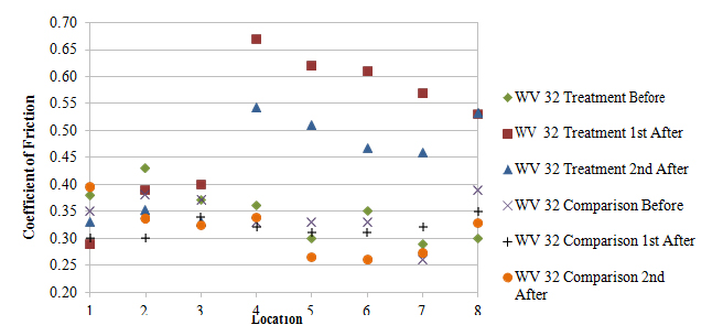
Figure 54. Graph. Side friction supply before and after for WV Route 32 sites.
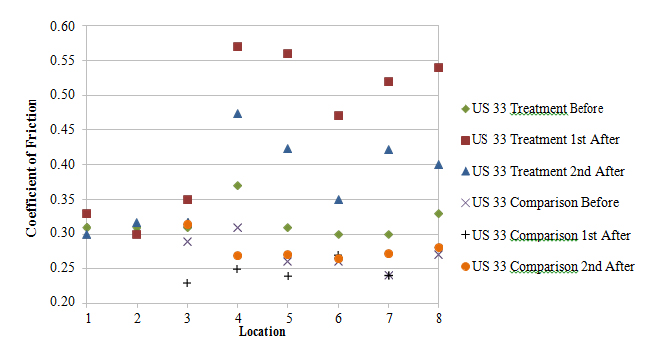
Figure 55. Graph. Side friction supply before and after for U.S. Route 33 sites.
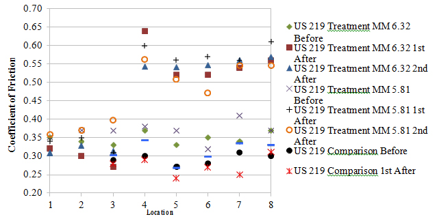
Figure 56. Graph. Side friction supply before and after for U.S. Route 219 sites.
In addition to the friction curves, the research team used speed data collected during the speed study to compute the difference in friction supply and the friction demanded by vehicles traversing horizontal curves at the treatment and control locations. The friction demand was computed using the point-mass model, using the equation shown in figure 57.

Figure 57. Equation. Side friction demand.
Where:
f = side friction demand
V = vehicle operating speed (mph)
R = radius of horizontal curve (ft)
e = rate of superelevation (percent).
During the friction testing, the research team used a digital slope meter to measure the superelevation at the midpoint of each horizontal curve. The research team also compared descriptive statistics from the distributions of friction demand (e.g., mean, SD, 95th percentile) at each treatment and control curve location with the friction supply distribution. Table 38 shows the descriptive statistics for each horizontal curve observed.
Table 38. Descriptive statistics for passenger cars for margin of safety analysis.
| Site | R |
e |
Passenger Car Speed |
Side Friction Supply |
||||||
Mean |
SD |
Min |
Max |
Mean |
SD |
Min |
Max |
|||
| WV Route 32 Treatment before | 680 |
8 |
48.05 |
5.64 |
27 |
67 |
0.32 |
0.03 |
0.29 |
0.36 |
| WV Route 32 Treatment 1st after | 680 |
8 |
46.54 |
5.13 |
23 |
58 |
0.60 |
0.05 |
0.53 |
0.67 |
| WV Route 32 Treatment 2nd after | 680 |
8 |
47.63 |
7.21 |
17 |
69 |
0.50 |
0.04 |
0.46 |
0.54 |
| WV Route 32 Comparison | 1073 |
7 |
52.76 |
7.62 |
30 |
72 |
0.33 |
0.05 |
0.26 |
0.39 |
| WV Route 32 Comparison 1st after | 1073 |
7 |
52.23 |
5.59 |
32 |
69 |
0.32 |
0.02 |
0.31 |
0.35 |
| WV Route 32 Compariosn 2nd after | 1073 |
7 |
52.48 |
6.06 |
24 |
75 |
0.32 |
0.05 |
0.26 |
0.40 |
| U.S. Route 33 Treatment before | 210 |
6 |
32.37 |
4.57 |
18 |
54 |
0.32 |
0.03 |
0.30 |
0.37 |
| U.S. Route 33 Treatment 1st after | 210 |
6 |
32.37 |
4.57 |
18 |
54 |
0.32 |
0.03 |
0.30 |
0.37 |
| U.S. Route 33 Treatment 2nd after | 210 |
6 |
30.15 |
15 |
54 |
0.41 |
0.04 |
0.35 |
0.47 |
0.31 |
| U.S. Route 33 Comparison | 265 |
8.5 |
36.17 |
6.79 |
13 |
58 |
0.27 |
0.03 |
0.24 |
0.31 |
| U.S. Route 32 Comparison 1st after | 265 |
8.5 |
35.46 |
6.09 |
12 |
48 |
0.26 |
0.01 |
0.24 |
0.28 |
| U.S. Route 32 Comparison 2nd after | 265 |
8.5 |
34.44 |
5.45 |
11 |
48 |
0.28 |
0.02 |
0.27 |
0.31 |
| U.S. Route 219 Treatment MM 6.32 before | 605 |
11 |
36.29 |
7.22 |
12 |
62 |
0.35 |
0.03 |
0.33 |
0.37 |
| U.S. Route 219 Treatment MM 6.32 1st after | 605 |
11 |
40.34 |
5.43 |
13 |
56 |
0.55 |
0.05 |
0.52 |
0.64 |
| U.S. Route 219 Treatment MM 6.32 2nd after | 605 |
11 |
41.97 |
4.72 |
30 |
63 |
0.55 |
0.01 |
0.54 |
0.57 |
| U.S. Route 219 Treatment MM 5.81 before | 273 |
12 |
34.80 |
6.73 |
21 |
66 |
0.37 |
0.03 |
0.32 |
0.41 |
| U.S. Route 219 Treatment MM 5.81 1st after | 273 |
12 |
37.14 |
6.46 |
21 |
70 |
0.58 |
0.03 |
0.56 |
0.61 |
| U.S. Route 219 Treatment MM 5.81 2nd after | 273 |
12 |
33.72 |
5.20 |
21 |
47 |
0.53 |
0.04 |
0.47 |
0.56 |
| U.S. Route 219 Comparison before | 545 |
12 |
41.16 |
4.35 |
29 |
53 |
0.29 |
0.01 |
0.27 |
0.31 |
| U.S. Route 219 Comparison 1st after | 545 |
12 |
43.86 |
5.35 |
26 |
54 |
0.27 |
0.03 |
0.24 |
0.31 |
| U.S. Route 219 Comparison 2nd after | 545 |
12 |
41.12 |
5.80 |
27 |
48 |
0.31 |
0.03 |
0.27 |
0.34 |
MM = Mile Marker
SD = Standard Deviation
Max = Maximum
Min = Minimum
The margin of safety, based on the difference between the distributions of friction supply and demand, was computed for each treatment and control location, as table 39 shows. The mean friction demand at all sites, for all time periods, is lower than the mean side friction supply. The 85th percentile friction demand at all treatment sites, for all time periods, except the before time period of the U.S. 33 treatment site, is lower than the mean side friction supply. The 85th percentile friction demand for all time periods of the U.S. 33 comparison site is greater than the side friction supply. The 95th percentile friction demand at all treatment sites, for all time periods except the before time period of the U.S. Route 33 treatment site, is lower than the mean side friction supply. The 95th percentile friction demand for all time periods of the U.S. Route 33 comparison site is greater than the side friction supply. The only additional site where the friction demand at the 95th percentile exceeded the friction supply was at the U.S. Route 219 treatment MM 5.81 site in the before period.
Table 39. Friction demand and supply comparison.
| Site | Side Friction Demand | Side Friction Supply | |||||
Mean |
85th Percentile |
95th Percentile |
Mean |
SD |
Min |
Max |
|
| WV Route 32 Treatment before | 0.146 |
0.205 |
0.242 |
0.321 |
0.034 |
0.290 |
0.360 |
| WV Route 32 Treatment 1st after | 0.132 |
0.183 |
0.216 |
0.598 |
0.053 |
0.530 |
0.670 |
| WV Route 32 Treatment 2nd after | 0.142 |
0.218 |
0.267 |
0.502 |
0.037 |
0.459 |
0.542 |
| WV Route 32 Comparison before | 0.103 |
0.159 |
0.195 |
0.329 |
0.045 |
0.260 |
0.390 |
| WV Route 32 Comparison 1st after | 0.099 |
0.139 |
0.164 |
0.322 |
0.022 |
0.310 |
0.350 |
| WV Route 32 Comparison 2nd after | 0.101 |
0.144 |
0.172 |
0.315 |
0.046 |
0.261 |
0.395 |
| U.S. Route 33 Treatment before | 0.273 |
0.377 |
0.445 |
0.321 |
0.033 |
0.300 |
0.370 |
| U.S. Route 33 Treatment 1st after | 0.238 |
0.319 |
0.371 |
0.533 |
0.040 |
0.470 |
0.570 |
| U.S. Route 33 Treatment 2nd after | 0.229 |
0.337 |
0.409 |
0.414 |
0.045 |
0.350 |
0.473 |
| U.S. Route 33 Comparison before | 0.244 |
0.385 |
0.479 |
0.268 |
0.026 |
0.240 |
0.310 |
| U.S. Route 33 Comparison 1st after | 0.232 |
0.354 |
0.435 |
0.257 |
0.014 |
0.240 |
0.280 |
| U.S. Route 33 Comparison 2nd after | 0.214 |
0.320 |
0.389 |
0.279 |
0.018 |
0.265 |
0.314 |
| U.S. Route 219 Treatment MM 6.32 before | 0.035 |
0.101 |
0.146 |
0.352 |
0.027 |
0.330 |
0.370 |
| U.S. Route 219 Treatment MM 6.32 1st after | 0.069 |
0.123 |
0.158 |
0.554 |
0.049 |
0.520 |
0.640 |
| U.S. Route 219 Treatment MM 6.32 2nd after | 0.084 |
0.132 |
0.162 |
0.552 |
0.012 |
0.540 |
0.569 |
| U.S. Route 219 Treatment MM 5.81 before | 0.176 |
0.306 |
0.394 |
0.372 |
0.028 |
0.320 |
0.410 |
| U.S. Route 219 Treatment MM 5.81 1st after | 0.217 |
0.349 |
0.438 |
0.583 |
0.026 |
0.560 |
0.610 |
| U.S. Route 219 Treatment MM 5.81 2nd after | 0.158 |
0.254 |
0.317 |
0.527 |
0.037 |
0.472 |
0.563 |
| U.S. Route 219 Comparison before | 0.087 |
0.135 |
0.166 |
0.288 |
0.013 |
0.270 |
0.310 |
| U.S. Route 219 Comparison 1st after | 0.115 |
0.179 |
0.220 |
0.272 |
0.030 |
0.240 |
0.310 |
| U.S. Route 219 Comparison 2nd after | 0.087 |
0.152 |
0.194 |
0.313 |
0.028 |
0.267 |
0.342 |
Bold indicates 85th percentile friction demand exceeded mean side friction supply.
Italics indicates 95th percentile friction demand exceeded mean side friction supply.
SD = Standard Deviation
Max = Maximum
Min = Minimum
Summary of HFST Evaluation Findings
The research team performed operational, driver behavior, and friction evaluations on four treatment and three corresponding comparison sites in West Virginia. The operational and driver behavior analyses generally found no consistent differences at the treatment sites between the before and after time periods from the data. The friction analysis, however, clearly demonstrated that the friction increased considerably at the four horizontal curve treatment locations in West Virginia. The friction generally remained high for 1year after the treatment was applied. A safety analysis being completed under a separate FHWA contract will reveal further information about the safety effects of the high-friction surface treatment.
1 The research team selected the point speed location before the curve to capture speeds that were unaffected by the HFST. The “upstream” location of 300 ft before the beginning of the treatment was based on 3.65 s of preview time at 55 mph (81 ft/s).