U.S. Department of Transportation
Federal Highway Administration
1200 New Jersey Avenue, SE
Washington, DC 20590
202-366-4000
Federal Highway Administration Research and Technology
Coordinating, Developing, and Delivering Highway Transportation Innovations
| REPORT |
| This report is an archived publication and may contain dated technical, contact, and link information |
|
| Publication Number: FHWA-HRT-14-020 Date: January 2015 |
Publication Number: FHWA-HRT-14-020 Date: January 2015 |
This section of the report describes a study to estimate the safety effects of lane width–shoulder width combinations on rural two-lane, two-way roads. This report first describes the background and study motivation. Next, it discusses the process for collecting safety data, including steps for identifying and defining segments, measuring geometric features, and gathering traffic and crash data. The research team then presents the statistical analysis methods for estimating the effects of lane and shoulder width allocation on both crash frequencies and severities; this is followed by the model estimation results and interpretation. The section concludes with a discussion of major findings and considerations for future research.
The conclusion that safety increases as lane width increases is based on the premise that wider lanes reduce the consequences of driver deviations from their intended path. Vehicles traveling in opposite directions on undivided, two-way roads are separated by larger distances if lanes are wider. Vehicles traveling in the same direction on multilane roads are also separated by larger distances if lanes are wider. Wider lanes provide more room for recovery in near-crash situations (e.g., evasive maneuvers to miss an object on the roadway or inadvertently drifting toward the roadside).
Using some of the same logic, it is also assumed that wider shoulders are associated with increased safety because they provide increased separation between a parked or disabled vehicle and the traveled way. Wider shoulders also provide more room for recovery following an unintentional (e.g., inattentive driver drift) or intentional (e.g., evasive maneuver) shoulder encroachment. Wider shoulders are also associated with larger lateral clearances from roadside objects and longer available sight distances when there are sight obstructions to the inside of horizontal curves.
Wider lanes and shoulders also appear to result in faster operating speeds.(47) For example, methodologies in the Highway Capacity Manual (HCM) predict an approximately 1.3 to 1.7 mph increase in speeds for every 1 ft increase in shoulder width on two-lane highways. Similarly, the HCM 2010 predicts an approximately 0.4 to 1.1 mph increase in speeds on two-lane highways for every 1 ft increase in lane width. (37) All else being equal, drivers traveling at faster speeds may be less likely to successfully react to unexpected situations (e.g., changes in lead vehicle behavior, non-motorized users crossing traveled way, changes in roadway alignment, roadside encroachments) than drivers traveling at slower speeds. In addition, the energy dissipated during a crash is directly proportional to the square of travel speed at the time of the crash. Impact forces that drivers experience increase as this initial speed increases and decreases as the time over which energy is dissipated decreases. The crash severity (i.e., probability of fatality or severe injury) therefore increases as initial travel speed increases.
The tradeoffs among speed, safety, lane width, and shoulder width are complex. Conclusions inferred from existing research are that wider cross sections tend to improve safety performance (i.e., fewer expected crashes); however, narrower cross sections tend to produce lower vehicle operating speeds. If these two points are independently true, then implementing reduced lane widths and shoulder widths as a speed management technique—a topic of interest for quite some time—should increase the number of crashes. However, some published safety studies indicate that there are cases where narrower cross sections are not necessarily associated with a higher expected crash frequency. For example, Gross et al. developed CMFs for lane-width–shoulder-width combinations on rural, two-lane highways.(48) The CMF estimation of interactions between lane width and shoulder width used a case-control methodology. Results yielded the following logical conclusions:
Rural, two-lane highway segments with lane-width–shoulder-width combinations totaling 16 to 17ft (e.g., 10-ft lanes with 6-ft shoulders; 11-ft lanes with 6-ft shoulders, 12-ft lanes with 5-ft shoulders) may not be any less safe than rural, two-lane highway segments meeting HSM base conditions (i.e., 12-ft lanes with 6-ft shoulders).
Bonneson and Pratt also estimated interactions between lane and shoulder width and drew similar conclusions—the safety effect of lane width depends on the shoulder width.(49) Research on lane width and safety on urban and suburban arterials, conducted as part of developing the HSM, concluded, “No consistent relationship was found between lane width and safety. Therefore, lane width was not included in the model.” (78) Other research on lane width in urban areas indicated that the “Broad lane indicator (lanes wider than 12 ft) was associated with a higher frequency of urban section run-off-road accidents. A plausible explanation is that a broader lane could be expected to allow a higher traveling speed and thereby create a greater likelihood for run-off-road [crashes] on urban sections”.(79)
The above-mentioned studies do have some limitations. For example, in the study by Gross et al. found the following:(48)
Harwood et al. did not report any model parameters for lane width, only the general conclusion about inconsistent relationships cited above.(78) No conclusive statements can be made to date other than considering lane width and shoulder width interactions appears to uncover cross-section combinations that will result in lower speeds (according to published speed prediction models) without a relative reduction in safety on rural two-lane roads. This is different than the current state-of-knowledge in the HSM and has the potential to contribute significantly to knowledge on geometric design, speed, and safety relationships and on the use of road geometry as a speed management technique.
Following a review of the literature conducted during an earlier task of this research, there was enough evidence for FHWA’s technical advisory team for this project to support exploring different combinations of lane and shoulder widths as a strategy to reduce operating speeds and improve safety on rural roads. This strategy has the potential to be low cost by reallocating existing pavement widths. This study focuses only on safety effects of lane-width–shoulder-width combinations. The study addresses the following limitations to previously published speed and safety research.
Most of the speed- and safety-related geometric design research reviewed in earlier tasks of this research focused on the effects of design elements in isolation and then combined the isolated effects through some additive or multiplicative process. This research looks at lane-width–shoulder-width combinations as opposed to isolated effects and used a variety of variable specifications for lane and shoulder widths, including indicator variables, continuous variables, and interaction terms.
Speed and safety prediction models reviewed in earlier tasks of this research were estimated by relating crashes and speed at some location to traffic, roadway, and other surrounding features at that same location (e.g., a short, homogenous segment). Proponents of self-enforcing, self-explaining roads have argued that the using cross-sectional geometry as a speed management technique will appear effective only when applied and studied over a significant stretch of road.(80) This research looks at the safety effects of lane widths and shoulder widths over significant stretches of road as opposed to short, homogenous segments. The research team used alignment indices to capture changes in alignment over these road segments.
Databases used to estimate models were verified and enhanced using satellite imagery from Google Earth™. The research team checked and confirmed or (when necessary) recoded with the correct measurement to verify accuracy of every attribute (e.g., lane width, shoulder width) in the electronically coded databases used for model estimation. In addition, the existing electronically coded databases were enriched by adding new attributes (e.g., curve radii; driveway density; barrier presence, length, and offset; roadside hazard rating; pavement markings) to lower the chances of omitted variable bias.
The research team explored the effects of lane-width–shoulder-width combinations on crash severity by estimating severity distribution functions (SDF) in addition to estimating different crash frequency models for various severity levels. The databases used to estimate the severity models contain the same crashes and road segments as the frequency model databases, but were restructured so that the basic observation unit (i.e., database row) is the crash instead of the road segment. The severity models can be used to estimate the probability, or proportion, of each severity level given the traffic, geometric, and traffic control characteristics. The newest HSM edition proposes methodologies for SDFs on freeways and interchanges, which appears to be a promising approach; however, to date, the applications in applied safety analysis are relatively limited.
The data collection effort focused on rural two-lane, two-way road segments in Minnesota and Illinois. The study did not include safety relationships at intersections or on intersection approaches. Rural areas were defined as those outside of urban boundaries, but not suburban. Suburban areas may be inside or outside urban boundaries. Some subjectivity was involved in defining an area as suburban.
The research initially identified three Highway Safety Information System (HSIS) States as possible data alternatives for this study: Illinois, Minnesota, and North Carolina. These three States were initially selected because of the availability of a number of precipitating event variables that could provide several alternatives for identifying a “speed-related crash” and data for roads classified “lower than” arterials (i.e., collectors and local roads). However, a majority of rural roads in North Carolina have unpaved shoulders, which would limit the ability to study different pavement allocations between lanes and shoulders. Thus, the research team considered only data from Minnesota and Illinois for the analysis. Initially, having access to multiple alternatives for identifying a “speed-related crash” was an important criterion because the safety results were to be linked with observational speed studies conducted along the same segments in the selected States. However, FHWA decided to focus on a more general safety study of lane-width–shoulder-width combinations and spend the remaining resources on more extensive field data collection for other treatments studied as part of this research effort (OSBs and high-friction surfaces).
The safety effects of lane-width–shoulder-width combinations were estimated through a cross-sectional study design for two reasons: 1) State and local transportation agencies do not routinely reallocate existing pavement widths, particularly in rural areas; and 2) the proportion of all possible lane-width–shoulder-width combinations that could be evaluated using a before–after study during this project, and their respective sample sizes, would be limited.
To overcome some of the documented limitations of cross-sectional study designs, such as those outlined in FHWA’s A Guide to Developing Quality Crash Modification Factors (FHWA-SA-10-32), the research team executed an in-depth, manual data collection effort to verify and enrich typical electronic databases often used for safety studies.(81) The research team also used modeling alternatives that address possible confounding factors between road segments with different lane-width–shoulder-width combinations not captured in the models (e.g., terrain, weather, driver characteristics, crash reporting thresholds, and practices). The following sections discuss these strategies.
Data Collection Sources, Tools, and Strategies
Data for this study included geometric features, traffic data, and crash data from rural roads. The research team used data collected from the following tools and information sources:
Database Verification and Enrichment
Safety models are commonly developed using electronically coded traffic and roadway data for independent variables; however, information in these datasets can be limited and inaccurate. Limited data means that the database may not include variables that could influence safety. Estimating safety models without these variables can result in omitted variable bias (i.e., erroneous parameter estimates for variables in the models). Including inaccurate information (e.g., incorrect dimensions for lane width) will result in biased parameter estimates. Based on this discussion, the research team applied the following techniques:
The research team used the aforesaid tools and techniques to conduct verification and enhancement activities.
The team used a combination of HSIS roadway data files, GIS roadway databases, and Google Earth™/Google Street View™ to collect roadway geometric characteristics. The team also manually defined each study segment. The segments were homogenous in terms of the number of lanes, lane width, shoulder width, shoulder type, and traffic volume. The segments did not include unsignalized or signalized intersections, and they began and ended at least 250 ft from adjacent intersections. The 250-ft number is consistent with research used to develop HSM predictive methods.(82)
The team explored different alignment indices to capture changes in horizontal alignment. This approach allowed longer segments to be defined in the database than those that would result from separating curves from tangents. Defining longer road segments was seen as a crucial step to determining whether geometry can be used to achieve desirable speed and safety effects. Most existing speed and safety prediction models relate crashes and speed at a specific location (e.g., a short, homogenous section) to traffic, roadway, and other surrounding features at that same specific location. The concept of driver expectancy recognizes that drivers make decisions based on previous experiences. Similarly, proponents of self-enforcing, self-explaining roads have argued that using geometry as a speed management technique appears effective only when applied and studied over a significant stretch of road.(80) Research to date has not captured this effect, but instead indicated that geometric design decisions made to reduce speeds (e.g., increased curvature, narrower lane widths) are expected to increase the expected number crashes.
The team defined road segments, collected their features and then checked and confirmed using Google Earth™’s satellite images and Google Street View™ photographs. The team used the Ruler tools in Google Earth™ to measure distances and to check and confirm lane width, shoulder width, segment length, and barrier presence and length. These tools were also used to measure deflection angles and horizontal curve lengths. The research team developed a set of Google Earth™ calculation tools to automate this process. NCHRP 17-45, Enhanced Safety Prediction Methodology and Analysis Tool for Freeways and Interchanges, used similar techniques.(83) The team also developed new tools compatible with the rural, two-lane context of interest for this current FHWA effort.
The first step of the data-collection process was locating the roadway segment of interest in Google Earth™ and determining its mileposts. Google Earth™ and other publicly available mapping and satellite imaging tools do not provide milepost information. However, the milepost of any point along a given State route in Minnesota and Illinois can be determined by using a combination of HSIS roadway data, GIS data for roadway networks, and Google Earth™. The following discussion provides a step-by-step description of the process. Any point along a route was identified by all three of the following identifiers:
HSIS roadway data files include all of these variables for both Illinois and Minnesota. The goal of this process was to then transfer these pieces of information from the HSIS roadway data files into Google Earth™ so the team could verify and enhance the data. HSIS data identified roadway segments by county, route number, and milepost. Google Earth™ uses coordinates. The team therefore used GIS data and ArcGIS™ software to translate location information from HSIS roadway inventory files into Google Earth™.
GIS roadway files from Illinois and Minnesota have different structures and information; therefore, the team could not use a single method of transferring HSIS data points into Google Earth™ through GIS for both States. Although there are many similarities, the procedure is described separately for Minnesota and Illinois. The procedure is illustrated by two examples, one for each State.
Minnesota Step 1: Collect route number, county number, and milepost from the HSIS roadway data file
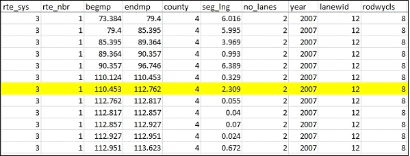
Figure 120 shows an example of the segment location information in the HSIS roadway data file for Minnesota. In this example, the beginning point of the segment shown in the seventh row is the point of interest. It is used throughout the process of locating this segment in Google Earth™. The point is located on Route 1, in County 4, at milepost 110.453.
Source: University of Utah
Figure 120. Chart. Location information in Minnesota’s HSIS Roadway File.
Minnesota Step 2: Locate the same point in Minnesota’s GIS roadway file and calculate its coordinates
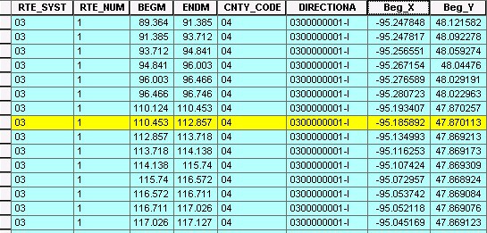
Minnesota’s GIS roadway data file also includes route number, county number, and milepost information. The point of interest (Route 1, County 4, Milepost 110.453) can be located and highlighted by opening the attribute table in ArcMap™ software. Figure 121 is a screenshot that illustrates this process. The eighth row (yellow-highlighted) has the beginning milepost of 110.453, the point of interest in this example. Two new columns named Beg_X and Beg_Y are created to store the x and y coordinates of the point (milepost 110.453). The team used the Calculate Geometry tool in ArcMap™ to transform the coordinate information of the point from its original NAD 1983 UTM (Zone 15N) to longitude and latitude in the WGS84 Coordinate System.
Source: University of Utah
Figure 121. Chart. Location information of the roadway segment in GIS File (Minnesota).
Minnesota Step 3: Locate and mark the point in Google Earth™
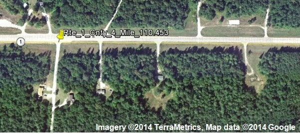
The team transferred the coordinates calculated from Step 2 into Google Earth™. A marker was placed at the location for future reference. Figure 122 is a screenshot of the point (MN Route 1, County 4, Milepost 110.453) located and marked with a place marker in Google Earth™.
 Original image: ©2014 Google®; annotations by University of Utah.
Figure 122. Photo. Locate and mark the point of interest in Google Earth™ using its coordinates (Minnesota).(84)
The above step-by-step process is systematically performed for all beginning points of the road segments on each route of interest in Minnesota. The coordinates of all points are then exported and automatically transferred into Google Earth™ using Keyhole Markup Language (KML) codes. The result of this process is a longitudinal reference system along each route in Google Earth™ with mileposts marked.
Illinois Step 1: Collect route number, county number, and milepost from the HSIS roadway data file
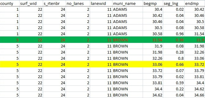
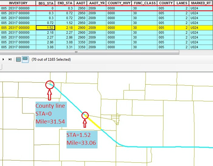
This step is very similar to Step 1 for Minnesota because the HSIS roadway data files from the two States have similar structures and identical information for county number, State route number, and milepost. However, GIS data files from Illinois do not have milepost information. Therefore, an additional piece of information is necessary for this step: the milepost of the route at the county line. The county line is then used as a reference point to calculate mileposts and locate all other points. Figure 123 shows an example of location information found in the Illinois HSIS roadway data file. Two rows in this figure are highlighted. The sixth row (green highlighted) is the first roadway segment on Route 24 in Brown County. The beginning milepost of this segment is the milepost of Route 24 at the county line (begmp = 31.54). Milepost 31.54 then becomes the reference point for all other points on Route 24 in Brown County. The beginning milepost of the tenth row (yellow highlighted) is the point of interest in this example. It is located in County 5 (Brown County), on Route 24, at milepost 33.06.
Source: University of Utah
Figure 123. Chart. Location information in Illinois HSIS Roadway data file.
Illinois Step 2: Locate the same point in Illinois GIS roadway file
Again, unlike Minnesota data, GIS files for the Illinois roadway network do not include milepost information. Illinois GIS files have two variables named BEG_STA and END_STA representing the stations (in units of mi) of beginning and ending points of each GIS roadway segment. (It should be noted that Illinois GIS deviates from standard surveying station measurements, which are usually in increments of 100 ft). Although actual milepost information is not available, the station can be used to compute the milepost of any point along the route. In most cases, BEG_STA=0.00 at the county line, and it increases west to east or south to north throughout the county. In some cases, the station resets back to 0.00 at some major intersecting points with other major routes.
The milepost of any given point on an Illinois route is computed using the equation shown in figure 124.

Figure 124. Equation. Reference point milepost.
Where:
Milepostref = the milepost of the reference point
STA = the station information (BEG_STA or END_STA) of the point in the GIS data file
In most cases, the milepost of the reference point is the milepost at the county line (determined in step 1). In some cases, it is the milepost of a major intersection where the beginning station (BEG_STA) resets back to 0.00. This reference point can be identified by looking through the attribute table of the GIS file and locating it using the same procedure as that used to compute mileposts.
While the direction of increasing milepost is the same as the direction of increasing station in the GIS files in most cases, they can be opposite in some rare instances. Because the distances are still the same, mileposts can be computed by reversing the direction of increasing station using the equation shown in figure 125.

Figure 125. Equation. Reference point milepost by reversing the direction of increasing station.
Where:
Milepostref = the milepost of the reference point
STAmax = the largest value of END_STA in the GIS file of a given county
STA = the station information (BEG_STA or END_STA) of the point in the GIS data file
Figure 126 shows an example of identifying the point of interest in this example. The first row of the data table indicates the county line with BEG_STA=0.00. The fifth row (yellow highlighted) shows the point of interest with a beginning station of 1.52 at milepost 33.06.
Source: University of Utah
Figure 126. Chart. Location information of the roadway segment in GIS file (Illinois).
Illinois Step 3: Determine the coordinates and locate the point in Google Earth™
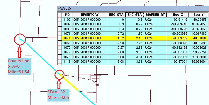
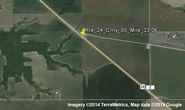
This step is similar to Minnesota step 2 and step 3. The research team used the Calculate Geometry tool in ArcGIS™ to coordinate each point in the WGS 1984 Coordinate System. Figure 127 shows the example of obtaining the coordinate information of milepost 33.06 (STA=1.52) along Illinois Route 24. The team then transferred the coordinates into Google Earth™, and the points were marked in the same way. Figure 128 is a Google Earth™ screenshot with the marker of milepost33.06.
Source: University of Utah
Figure 127. Chart. Identify coordinate information associated with the roadway segment (Illinois).
Original image: ©2014 Google®; annotations by University of Utah.
Figure 128. Photo. Locate and mark the roadway segment in Google Earth™ with its coordinates.(85)
Following the steps outlined above, the research team created a series of mile markers in Google Earth™—creating a longitudinal reference system along each route. The team then explored each route over the 3 years of the analysis period (2007, 2008, 2009) to determine the candidate study segments. In the process, the team also checked whether there were any significant changes to the route (indicating a possible reconstruction project that changed milepost definitions). The team used historical satellite imagery (in Google Earth™) and crash data codes to eliminate sections of roadway with work zones during the analysis period. The team selected and marked candidate study segments based on the following three criteria:
Through this process, the team retained only longer segments (about 0.5 mi and longer). As explained above, the purpose of using the longer segments is to address a limitation of previous studies and capture results regarding the proposed idea that using geometry as a speed management technique will appear effective from a safety perspective only when applied and studied over a significant stretch of road.
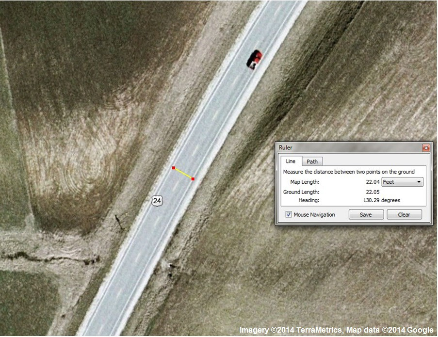
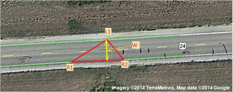
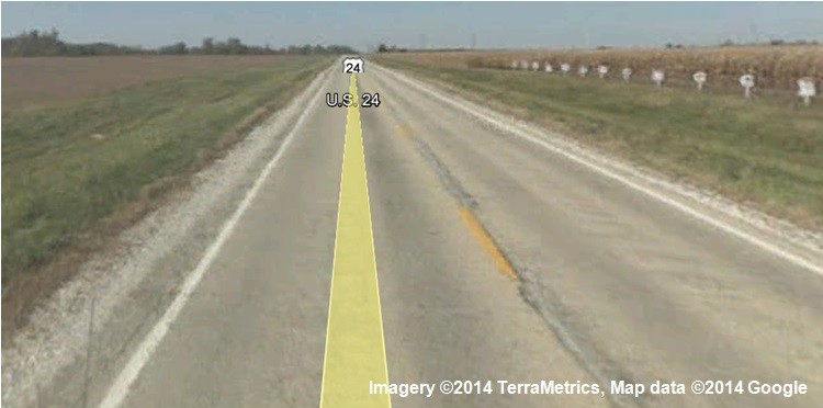
Using the HSIS roadway files, the research team had a basic idea of the lane configuration (i.e., number of through lanes and auxiliary lane present), lane width, shoulder width, and shoulder types. The team then used a combination of Google Earth™ satellite images and a set of Google Earth™ calculation tools created by the research team using Visual Basic for Applications (VBA) in Microsoft™ Excel to check these features at incremental distances along the defined segments. Figure 129, figure 130, and figure 131 are screenshots of Google Earth™ and Google Street View™ illustrating the procedure. The team tested the accuracy of the Google Earth™ measurements of widths using Google Earth™’s distance measurement tools to take measurements of known distances (e.g., football field markings), which were found to be accurate. The determination of lane width was partly automated by developing VBA codes to continuously calculate the height of a moving triangle along each segment. Two points on one edge line and another on the opposite edge of the road form the triangle. Figure 131 illustrates this concept.
Original image: ©2014 Google®; annotations by University of Utah.
Figure 129. Photo. Measurement of cross-section features in Google Earth™.(86)
Original image: ©2014 Google®; annotations by University of Utah.
Figure 130. Photo. Conceptual illustration of calculating lane.(87)
Original image: ©2014 Google®; annotations by University of Utah.
Figure 131. Photo. Visual checks of cross-section features in Google Street View™.(88)
Other roadside elements may also influence safety and should be controlled for when trying to determine the safety effects of lane-width–shoulder-width combinations. These include barrier presence, barrier length and offset (from the travel lane), type of center line and edge line markings, number of driveways, and the roadside hazard rating. The team adopted the roadside hazard rating developed by Zegeer et al. and currently used in the HSM predictive method for rural, two-lane roads for this study.(89) The team collected these data elements and then coded for the defined segments.
Table 97 provides a summary of the dataset by cross-section configuration with the number of roadway segments by each lane-width and shoulder-width category.
Table 97. Number of segments by lane-width and shoulder-width.
| Lane Width (ft) | Shoulder Width (ft) | State | Total | |
| Illinois | Minnesota | |||
| 10 | All | 55 | 6 | 61 |
| 0–3 | 38 | 0 | 38 | |
| 4–6 | 15 | 2 | 17 | |
| > 6 | 2 | 4 | 6 | |
| 11 | All | 267 | 81 | 348 |
| 0–3 | 109 | 9 | 118 | |
| 4–6 | 142 | 16 | 158 | |
| > 6 | 16 | 56 | 72 | |
| 12 | All | 219 | 249 | 468 |
| 0–3 | 57 | 28 | 85 | |
| 4–6 | 126 | 53 | 179 | |
| > 6 | 36 | 168 | 204 | |
| 13 | All | 0 | 9 | 9 |
| 0–3 | 0 | 6 | 6 | |
| 4–6 | 0 | 1 | 1 | |
| > 6 | 0 | 2 | 2 | |
| Total | 541 | 345 | 886 | |
Table 98 provides a summary of the dataset by the presence of roadside barriers; table 99 shows the presence of driveways.
Table 98. Number of segments with roadside barriers.
| Roadside Barriers | State | Total | |
| Illinois | Minnesota | ||
No | 416 | 300 | 716 |
Yes | 125 | 45 | 170 |
Total | 541 | 345 | 886 |
Table 99. Number of segments by driveway presence.
| Number of Driveways | State | Total | |
| Illinois | Minnesota | ||
| 0 | 134 | 95 | 229 |
| 1–10 | 368 | 242 | 610 |
| 11–20 | 30 | 8 | 38 |
| > 20 | 9 | 0 | 9 |
| Total | 541 | 345 | 886 |
A limitation of previous studies of lane-width–shoulder-width combinations was the lack of control for horizontal curvature, particularly if the data were from States other than Washington. Horizontal curve data are not available in most roadway inventory databases, but these data are crucial to modeling safety performance along rural and suburban roads. The research team used a combination of Google Earth™ path-marking tools and custom-made Google Earth™ calculation tools developed using VBA in Microsoft™ Excel to collect data for each horizontal curve on the defined road segments. The method was developed and tested using horizontal curves of known geometry and found to be accurate (i.e., measured and actual radius within approximately 2.5 percent). The following steps illustrate this technique, which measures the deflection angle and long chord.
Step 1: Place a path on the centerline. Use the Add path tool in Google Earth™ to trace along the centerline of roadway. This path needs to cover the entire curve and extend to partly cover both tangent lines. This path is visually placed and adjusted so that it matches the centerline of the roadway as closely as possible (see figure 132).
Step 2: Export the overlaid Google Earth™ path and extract the coordinate information. The path is then exported from Google Earth™ into a KML file. The KML file holds coordinate information of points along this path. These coordinates are then extracted using VBA codes specifically developed for this task. A computer algorithm also developed specifically for this task detects and categorizes these points into those on the curve and those on the two tangents based on their coordinates and positions relative to each other.
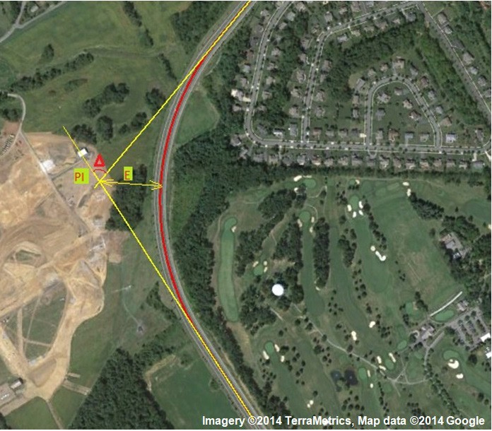
Step 3: Develop straight-line equations for the tangents and compute the deflection angle. The VBA program then uses the coordinates of the points on the tangents to compute two straight-line equations through linear regression. The coordinates of point of intersection (PI) and the deflection angle (Δ) are then computed from these two straight-line equations.
Original image: ©2014 Google®; annotations by University of Utah.
Figure 132. Photo. Screenshot of estimating deflection angles in Google Earth™.(90)
Step 4: Calculate external distance E, radius R, and length of curve L. With the coordinates of the PI known, a minimization algorithm determines the smallest distance between the PI and the curve. The computer code searches for the smallest distance between the PI and all points along the curve using the equation shown in figure 133.

Figure 133. Equation. Smallest distance between PI and all points along the curve.
The curve radius is then calculated using the equation shown in figure 134.
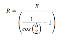
Figure 134. Equation. Curve radius.
The length of the curve is then calculated using the equation shown in figure 135.

Figure 135. Equation. Length of the curve.
This four-step process is applied to every horizontal curve along the defined study segments. The team explored alignment indices to capture changes in horizontal alignment to define longer segments with multiple curves in the database. The advantages of this approach are discussed earlier in this section. Table 100 provides alternative indices explored as ways to quantify the horizontal alignment characteristic of each extended road segment. These are based on a previous study that attempted to use alignment indices to predict operating speeds.(91) It is important to note that the objective of this study is not to estimate the effects of the alignment indices on speed and safety, but to control for horizontal alignment characteristics on extended lengths of road while studying the effects of lane-width–shoulder-width combinations.
Table 100. Alignment indices for quantifying horizontal alignment characteristics (based on Fitzpatrick et al., 2000).(91)
| Horizontal Alignment Index | Formula |
| Curvature Change Rate (CCR) (degrees/mi) | 
Where: |
| Degree of Curvature (DC) (degrees/mi) | 
Where: |
| Curve Length: Roadway Length (CL:RL) | 
Where: |
| Average Radius—AVG R (ft) | 
Where: |
| Average Tangent—AVG T (ft) | 
Where: |
The research team also used maps with area type boundaries combined with the Google Earth™ images and Google Street View™ photography to collect other variables that describe the road segment. These include area type (rural, rural transition zone, rural community, suburban), presence and type of edge line and centerline markings, and presence of shoulder and/or centerline rumble strips.
Table 101 shows a summary of the dataset by the presence of no-passing zone (solid centerline), one-directional passing zone (one-sided solid centerline), and the presence of shoulder rumble strips. Rumble strip information was initially included in the model. However, most of the segments with shoulder rumble strips are in Minnesota so the rumble strip variable is correlated with the State indicator. Therefore, the research team dropped rumble strips from the model, and the State indicator likely captured its effects.
Table 101. Number of segments with no-passing zone, one-sided passing zone, and shoulder rumble strip.
| Segment Characteristics | State | Total | ||
| Illinois | Minnesota | |||
| No Passing (Solid centerline) | No | 382 | 272 | 654 |
| Yes | 159 | 73 | 232 | |
| Total | 541 | 345 | 886 | |
| One-Sided Passing (One-sided solid centerline) | No | 246 | 164 | 410 |
| Yes | 295 | 181 | 476 | |
| Total | 541 | 345 | 886 | |
| Shoulder Rumble Strip | No | 536 | 180 | 716 |
| Yes | 5 | 165 | 170 | |
| Total | 541 | 345 | 886 | |
The team collected traffic volumes from the HSIS database. Traffic volume was one of the variables used to define a homogenous roadway segment. The team defined traffic volume for each roadway segment for each of the three analysis years (2007, 2008, 2009).
Table 102 provides descriptive statistics for the geometric, traffic control, and traffic variables that describe the 886 rural, two-lane highway segments observed for this study. Ultimately, the approximately 1 percent of segments (a total of 9 segments) with lane widths equal to 13 ft were deleted from the database used for model estimation, resulting in 877 total segments.
Table 102. Descriptive statistics for geometric, traffic control, and traffic variables.
| Variablea | Number of Observation | Mean | Standard Deviation | Minimum | Maximum |
| aadt | 886 | 3,436.54 | 2,353.04 | 450 | 19,190 |
| ln_aadt | 886 | 7.93 | 0.67 | 6.11 | 9.86 |
| seglen | 886 | 0.82 | 0.41 | 0.11 | 2.92 |
| illinois | 886 | 0.61 | 0.49 | 0 | 1 |
| Lane10 | 886 | 0.07 | 0.25 | 0 | 1 |
| Lane11 | 886 | 0.39 | 0.49 | 0 | 1 |
| Lane12 | 886 | 0.53 | 0.50 | 0 | 1 |
| Lane13 | 886 | 0.01 | 0.10 | 0 | 1 |
| shoulder | 886 | 5.29 | 2.78 | 0 | 12.00 |
| ln10shld | 886 | 0.22 | 1.02 | 0 | 9.00 |
| ln11shld | 886 | 1.84 | 2.79 | 0 | 12.00 |
| barrier | 886 | 0.01 | 0.02 | 0 | 0.36 |
| drvwy_den | 886 | 3.93 | 5.40 | 0 | 63.41 |
| solid_CL | 886 | 0.07 | 0.17 | 0 | 1.13 |
| dash1_CL | 886 | 0.10 | 0.12 | 0 | 0.50 |
| curve | 886 | 0.30 | 0.46 | 0 | 1 |
aThe following are the variable definitions:
aadt = Average annual daily traffic (vehicles/day)
ln_aadt = Natural logarithm of aadt
seglen = Segment length (mi)
illinois = Indicator for State in which the road segment is located (=1 if the data is from Illinois; =0 if the data is from Minnesota)
Lane10 = Indicator for 10-ft lane width (=1 if the segment has a 10-ft lane width; =0 otherwise)
Lane11 = Indicator for 11-ft lane width (=1 if the segment has a 11-ft lane width; =0 otherwise)
Lane12 = Indicator for 12-ft lane width (=1 if the segment has a 12-ft lane width; =0 otherwise)
Lane13 = Indicator for 13-ft lane width (=1 if the segment has a 1-ft lane width; =0 otherwise)
shoulder = Total shoulder width, both paved and unpaved shoulders (ft)
ln10shld = Interaction between 10-ft lane and shoulder width (=Lane10*Shoulder)
ln11shld = Interaction between 11-ft lane and shoulder width (=Lane11*Shoulder);
barrier = Length and offset of roadside barrier (=barrier_length/(barrier_offset*total_segment_length)
drwy_den = Driveway density (=number_of_driveways/total_segment_length)
solid_CL = Variable representing the proportion of no-passing zone (= total_length_of_solid_center_line/total_segment_length)
dash1_CL = Variable representing the proportion of one-sided passing zone (=total_length_of_one-sided_solid_center_line/total_segment_length)
curve = Indicator variable representing the horizontal alignment (=1 if the total sum of (radius/deflection angle) falls between 10 and 1,000; =0 otherwise).
The team collected crash data from the HSIS crash databases. After defining all study segments and determining their beginning and ending mileposts, the team counted the number of crashes that occurred within each segment. The team used 3 years of crash data (2007, 2008, 2009) for the safety analysis in this study. The team also counted the following crash types on each road segment:
Table 103 provides descriptive statistics for the crash variables.
Within the total and fatal-plus injury crash levels, the team explored crash severity in greater detail because of the expected interaction among lane width, shoulder width, and speed discussed in the background section. The team estimated SDFs for the total and fatal-plus-injury crashes using multinomial logit models (discussed at greater depth in the following section). The databases used to estimate the severity models consisted of the same crashes, road segments, and variables as the frequency model databases, but were restructured so the basic observation unit (i.e., database row) is the crash instead of the road segment.
Table 103. Descriptive statistics for crash variables.
| Variable | Number of Observation | Mean | Standard Deviation | Minimum | Maximum |
| tot_all | 886 | 2.71 | 3.55 | 0 | 32 |
| sv_all | 886 | 2.27 | 3.21 | 0 | 31 |
| mv_all | 886 | 0.44 | 0.94 | 0 | 10 |
| key_kabco | 886 | 2.94 | 4.01 | 0 | 35 |
| sv_fi | 886 | 0.31 | 0.66 | 0 | 6 |
| mv_fi | 886 | 0.17 | 0.47 | 0 | 4 |
| key_kabc | 886 | 0.57 | 1.14 | 0 | 10 |
| sv_o | 886 | 1.95 | 2.96 | 0 | 28 |
| mv_o | 886 | 0.27 | 0.71 | 0 | 7 |
| key_o | 886 | 2.38 | 3.49 | 0 | 30 |
The following are the variable definitions:
tot_all = Total crashes (all types and severities)
sv_all = Single-vehicle crashes (all severities)
mv_all = Multiple-vehicle crashes (all severities)
key_kabco = Key lane width/shoulder with crashes (all severities) that include single-vehicle-run-off-road and multiple vehicle head-on, sideswipe opposite direction, and sideswipe same direction
sv_fi = Single-vehicle crashes (fatal-plus-injury)
mv_fi = Multiple-vehicle crashes (fatal-plus-injury)
key_kabc = Key lane width/shoulder with crashes (fatal-plus-injury)
sv_o = Single-vehicle crashes (property damage only (PDO))
mv_o = Multiple-vehicle crashes (PDO)
key_o = Key lane width/shoulder with crashes (PDO)
Safety Data Analysis Methodologies
Analysis of Expected Crash Frequency
The team used negative binomial regression modeling to explore the effects of lane-width–shoulder-width combinations on expected crash frequency. The team estimated the full regression models that consider all the variables collected, in addition to lane width and shoulder width, to reduce the possibility of omitted variable bias. In the negative binomial model, the expected number of crashes of type i on segment j is typically expressed using the equation shown in figure 136.
\
Figure 136. Equation. Expected number of crashes of type i on segment j.
Where:
μij= E(Yij ) = the expected number of crashes of type i on segment j
Xj = a set of traffic and geometric variables characterizing segment j
β = regression coefficients estimated with maximum likelihood that quantify the relationship between E(Yij)and variables in X
Lj = length of segment j
Ln(Lj ) = the natural logarithm of segment length

Figure 137. Equation. Variance of crashes of type i on segment j.
Where:
VAR(Yij ) = variance of crashes of type i on segment j
E(Yij ) = the expected number of crashes of type i on segment j
α = overdispersion parameter
The research team explored both constant overdispersion parameters as well as overdispersion parameters that apply to a unit length of road when estimating the lane-width and shoulder-width models. Ultimately, they selected models with a constant overdispersion parameter.
The research team explored variations of the negative binomial model to address crash-influencing factors that may be common to groups of road segments, but that are not captured by the models. Failure to address these factors during model estimation may result in biased parameter estimates and underestimated standard errors. Hauer classified these factors as “unrecognized, or not understood, or unmeasured.”(92) Examples include terrain type, weather, and crash-reporting thresholds of the agency overseeing a particular area. The latter can be particularly important in estimating safety performance functions for less severe (e.g., PDO) crashes.
Negative binomial models with identification variables for counties, districts, regions, or States treated as fixed or random effects are modeling alternatives to address these “shared unobservables.” The fixed effects estimator has less restrictive assumptions, but it is not always useful if the independent variables of interest do not vary within the fixed effects (e.g., if a particular county had the same lane width throughout, then the fixed effects for that county and lane width could not both be included in the model). The random effects estimator addresses this challenge, but is only appropriate if the random effects are not correlated with the independent variables in the model. This assumption can be investigated with a Hausman test.(93) The models reported in this report ultimately implemented a fixed effects approach with indicator variables representing State (i.e., 1 = Illinois, 0 = Minnesota).
The research team tested the effects of lane-width–shoulder-width combinations through a number of variable specifications. It has been common to include lane width and shoulder width in a linear specification. However, the team also explored the inverse of lane width and shoulder width in an attempt to capture an increased effect of lane width and shoulder width on safety when widths are narrow. As the widths become wider and wider, the safety effects diminish. The team also tested indicator variables for lane-width–shoulder-width combinations. Indicator variables capture possible nonlinear or noncontinuous relationships. In the end, the research team settled on specifications of indicator variables for lane widths, shoulder width as a continuous variable in a linear specification, and interactions between the lane-width indicator variables and shoulder width to capture the varying effects of lane-width–shoulder-width combinations.
Accurate predictions of crash severity are important when looking at combinations of lane widths and shoulder widths. Severity distributions may change significantly with cross-section allocation through a resulting increase or decrease in operating speeds. Severity distributions are likely to vary differently with traffic volumes and design decisions depending on crash type (e.g., single vehicle or multiple vehicle). The research team used logit models to estimate an SDF to address these issues. The logit models produce the probabilities (or proportions) of crash severity outcomes as a function of traffic volume, geometry, and other road characteristics. The multinomial logit, nested logit, and ordered outcome models are possible model alternatives.(94,95,96) The databases used to estimate the severity models consist of the same crashes road segments and variables as the frequency model databases, but restructured so that the basic observation unit (i.e., database row) is the crash instead of the road segment. The frequency models and SDFs can be combined to estimate the number of accidents of different severity levels.(97)
For this research, the research team used the multinomial logit model to estimate SDFs within the total and fatal-plus-injury crash levels. In the multinomial logit model, the probability that accident n will have severity i is expressed using the equation shown in figure 138.

Figure 138. Equation. Probability of accident n with severity i.
Where Xn is a set of variables that will determine the crash severity, and βi is a vector of parameters to be estimated. The same factors specified in the frequency models were also specified in the severity models, including variables for different lane-width–shoulder-width combinations at the crash location.
Model Estimation Results and Discussion
All models were estimated using STATA® 12.1, created by StataCorp, located in College Station, TX. Table 104 and table 105 provide negative binomial regression model estimation results for total crashes (all types and severities) fatal-plus-injury crashes (all types), respectively. Appendix C provides model estimation results for other crash types (as outlined in the Crash Data section).
Table 104. Negative binomial regression model estimation results for total crashes (all types and severities).
| Variable | Coefficient | Standard Error | z | P > z | 95-Percent | |
| ln_aadt | 0.652 | 0.053 | 12.25 | < 0.001 | 0.547 | 0.756 |
| illinois | 0.994 | 0.092 | 10.78 | < 0.001 | 0.813 | 1.175 |
| Lane10 | 0.985 | 0.201 | 4.89 | < 0.001 | 0.590 | 1.380 |
| Lane11 | 0.489 | 0.146 | 3.34 | 0.001 | 0.202 | 0.775 |
| shoulder | -0.042 | 0.021 | -1.97 | 0.048 | -0.083 | 0.000 |
| ln10shld | -0.119 | 0.053 | -2.25 | 0.024 | -0.222 | -0.016 |
| ln11shld | -0.052 | 0.028 | -1.88 | 0.060 | -0.106 | 0.002 |
| barrier | 3.925 | 1.593 | 2.46 | 0.014 | 0.803 | 7.047 |
| drvwy_den | 0.014 | 0.006 | 2.32 | 0.020 | 0.002 | 0.025 |
| solid_CL | 0.517 | 0.188 | 2.75 | 0.006 | 0.149 | 0.886 |
| dash1_CL | 0.862 | 0.293 | 2.94 | 0.003 | 0.288 | 1.437 |
| curve | 0.224 | 0.067 | 3.35 | 0.001 | 0.093 | 0.355 |
| _cons | -5.041 | 0.424 | -11.89 | < 0.001 | -5.872 | -4.210 |
| ln(Length) | 1 | (exposure) | N/A | N/A | N/A | |
| /lnalpha | -1.129 | 0.117 | N/A | N/A | -1.358 | -0.900 |
| alpha | 0.323 | 0.038 | N/A | N/A | 0.257 | 0.406 |
Log Likelihood = -1608.0603
Number of Observations = 877
LR chi2(12) = 443.79
Prob > chi2 = 0
Pseudo R2 = 0.1213
Likelihood-ratio test of alpha=0: chibar2(01) = 239.90 Prob>=chibar2 = 0.000
N/A = Not Available
Table 105. Negative binomial regression model estimation results for fatal-plus-injury crashes (All types).
| Variable | Coefficient | Standard Error | z | P > z | 95-Percent Confidence Interval |
|
| ln_aadt | 0.736 |
0.092 |
7.980 |
< 0.001 |
0.555 |
0.917 |
| illinois | 0.426 |
0.151 |
2.830 |
0.005 |
0.131 |
0.721 |
| Lane10 | 0.315 |
0.384 |
0.820 |
0.412 |
-0.437 |
1.066 |
| Lane11 | 0.424 |
0.259 |
1.640 |
0.101 |
-0.083 |
0.932 |
| shoulder | -0.016 |
0.035 |
-0.450 |
0.650 |
-0.085 |
0.053 |
| ln10shld | -0.047 |
0.093 |
-0.500 |
0.615 |
-0.228 |
0.135 |
| ln11shld | -0.063 |
0.047 |
-1.330 |
0.183 |
-0.156 |
0.030 |
| barrier | 2.370 |
2.552 |
0.930 |
0.353 |
-2.631 |
7.372 |
| drvwy_den | 0.002 |
0.010 |
0.170 |
0.866 |
-0.019 |
0.022 |
| solid_CL | 0.453 |
0.311 |
1.460 |
0.145 |
-0.156 |
1.062 |
| dash1_CL | 0.404 |
0.499 |
0.810 |
0.419 |
-0.575 |
1.383 |
| curve | 0.113 |
0.113 |
1.000 |
0.316 |
-0.108 |
0.335 |
| _cons | -6.856 |
0.738 |
-9.290 |
< 0.001 |
-8.303 |
-5.409 |
| ln(Length) | 1 |
(exposure) |
N/A |
N/A |
N/A |
N/A |
| /lnalpha | -1.49881 |
0.464812 |
N/A |
N/A |
-2.40983 |
-0.5878 |
| alpha | 0.223396 |
0.103837 |
N/A |
N/A |
0.089831 |
0.55555 |
Log Likelihood = -744.43799
Number of Observations = 877
LR chi2(12) = 94.08
Prob > chi2 = 0.000
Pseudo R2 = 0.059
Likelihood-ratio test of alpha=0: chibar2(01) = 6.69 Prob>=chibar2 = 0.005
N/A = Not Available
For the total crash model, all model parameters except one were statistically significant at a 95‑percent confidence level (i.e., with a probability of a Type I error less than 5 percent). The p-value for the interaction of the 11-ft lane width indicator and shoulder width indicated a 6‑percent chance of a Type I error. Parameter signs were all generally in the direction expected. Parameters for lane width indicators showed that, with shoulder width ignored, the expected number of total (i.e., all types and severities) crashes increases as lane width decreases. The main effect of shoulder width was a decrease in the expected number of crashes as shoulder width increased. In addition, the interaction of the lane width indicator and shoulder width showed that shoulder width has the greatest effect on safety when the lane width equals 10-ft. Shoulder width also has a greater effect on safety when the lane width is 11-ft than when the lane width is 12-ft. Figure 139 shows these findings are demonstrated in the form of CMFs.
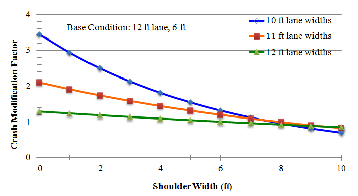
Figure 139. Graph. CMFs for lane-width–shoulder-width combinations developed directly from regression model parameters, total crashes (all types and severities) on rural, two-lane roads (developed from model estimation results in table 104).
For the fatal-plus-injury crashes, only the 11-ft lane width indicator, the 11-ft lane width, and shoulder width interaction were statistically significant at a level higher than 80 percent among the cross-section variables. Parameter signs were all generally in the direction expected, with the same signs as the total crash model parameters. Parameters for lane width indicators showed that, with shoulder width ignored, the expected number of fatal-plus-injury crashes (all types) increases as lane width decreases, but it is difficult to distinguish the performance of an 11-ft lane width from a 12-ft lane width. The main effect of shoulder width was a decrease in the expected number of fatal-plus-injury crashes as shoulder width increased, but the probability of a Type I error was quite high (near 65 percent). The interaction of the lane width indicator and shoulder width showed that shoulder width has additional, positive effects on safety when the lane width is less than 12 ft. Figure 140 shows that these findings are demonstrated in the form of CMFs.
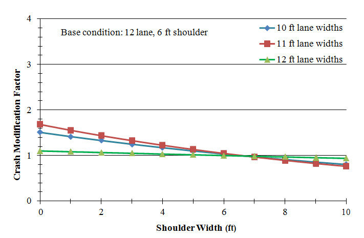
Figure 140. Graph. CMFs for lane-width–shoulder-width combinations developed directly from regression model parameters, fatal-plus-injury crashes (all types) on rural, two-lane roads (developed from model estimation results in table 105).
The results discussed above show more complex (but intuitive) interactions between expected crash frequency, lane width, and shoulder width than what is currently reflected in the Highway Safety Manual CMFs. For any given pavement width, there are combinations of lane width and shoulder width that result in the lowest expected crash frequency (for all crash types and severities as well as for fatal-plus-injury crashes). For narrower total paved widths, the optimal lane width appears to be 12 ft. This general conclusion is consistent with conclusions from Gross et al.(48) As total paved widths become larger, there is not necessarily a safety benefit from using a wider lane, and in some cases, using a narrower lane appears to result in lower than expected crash frequencies.
One possible explanation continues to be likely differences in operating speeds for different lane-width–shoulder width combinations. Initially, these safety results were to be linked with observational speed studies conducted along selected Illinois and Minnesota segments to confirm this hypothesis. However, FHWA officials decided to focus on a more general safety study of lane-width–shoulder-width combinations and spend the remaining resources on more extensive field data collection for other treatments studied as part of this research effort (OSBs and high-friction surfaces).
Appendix C provides the multinomial logit model estimation results for total crashes (all types and severities) with property damage only set as the base outcome, and fatal-plus-injury crashes (all types) with possible injury crashes set as the base outcome. This was done in an effort to estimate SDFs in addition to estimating different crash frequency models for various severity levels. The databases used to estimate the severity models consisted of the same crashes and road segments as the frequency model databases, but restructured so the basic observation unit (i.e., database row) is the crash instead of the road segment. The newest Highway Safety Manual proposes SDFs in methodologies on freeways and interchanges.
The SDFs do not show statistically significant and consistent results in terms of the geometric effects on crash severity defined in this way. This is not necessarily surprising, given that the interpretation of these models is “the probability of a severity outcome, given that a crash has occurred.” The geometric features are not expected to directly influence the severity outcome given that the crash has occurred; geometric features are likely to influence the likelihood of the crash occurring. Vehicle- and occupant-related characteristics, as well as the characteristics of a given collision, are much more likely to influence this conditional severity outcome. The finding indicates the need for additional exploration of SDFs and their sensitivity to road design and traffic control features.