U.S. Department of Transportation
Federal Highway Administration
1200 New Jersey Avenue, SE
Washington, DC 20590
202-366-4000
Federal Highway Administration Research and Technology
Coordinating, Developing, and Delivering Highway Transportation Innovations
| REPORT |
| This report is an archived publication and may contain dated technical, contact, and link information |
|
| Publication Number: FHWA-HRT-10-035 Date: September 2011 |
Publication Number: FHWA-HRT-10-035 Date: September 2011 |
The developed ANN models were ranked based on the performance of each model for an independent dataset that contains all of the required input parameters to be used in the different models. The decision tree in figure 60 is the result of this prioritization and was used to populate the LTPP database. As suspected at the outset of this project, the MR ANN model yields the best prediction possible and is the preferred model. This finding is not surprising given that the MR ANN model takes actual mixture measured quantities as input. The intuition is also supported in the fitting statistics shown in the figures presented in section 5.0. If MR data are not available, the next preferred model is the VV ANN model. Although the VV ANN shows poorer fitting statistics than the GV ANN model in terms of logarithmic space, it shows better statistics in terms of arithmetic space. The arithmetic statistics were used to rank these models because the moduli values are expressed and utilized in terms of their arithmetic value. Of the three ANN models, GV ANN received the lowest ranking. However, GV-PAR outranked the VV-grade because the model GV-PAR uses measurements taken directly from the material of interest. The VV-grade model uses viscosity values representative of the binder grade.
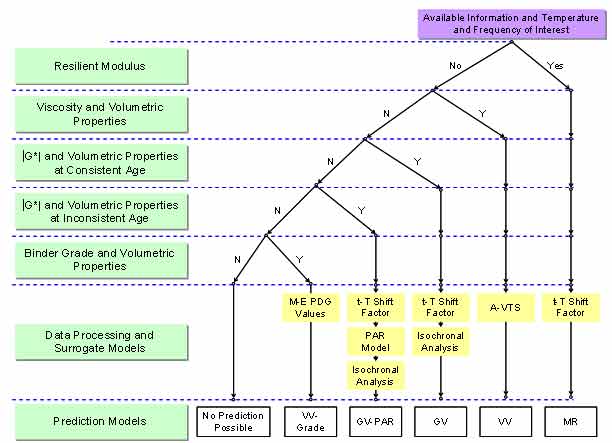
Figure 60. Illustration. Decision tree applied to population of LTPP database based on ranking of ANN models.
The input sets available for each section are different. Consequently, the models that can be utilized for a given section may differ. All the models that can be used for a specific section have been identified. If any of the inputs are outside the range of the calibration data, then the model for that section is considered to be a violated model, and predictions with it may or may not be reasonable. Any available model that does not violate the input range criteria is used as the predictive model for that section. In cases where only two violated models are available, the model for that section must be decided manually by the user.
Two sets of internal QC checks were applied to the |E*| data produced for submission to the LTPP database. The first QC check was used on the input values. All the other QCs were used to check the output |E*| predictions. In the following sections, each of these QC criteria is described. The work criterion is implied but not explicitly stated for each of these checks. The quality grading system referenced is different than the standard record status definition used in the LTPP database. For example, data assigned an “A” by the research team represent the highest quality data, whereas the LTPP convention assigns an “E” to the highest quality data. The research team established strict QC checks for these data to ensure that only the highest quality data were assigned an “A” grade. The data that did not achieve an “A” grade should be used with caution, and users should be fully aware that the data did not pass the QC check. All predictions are included in the database so users can determine whether or not the data are suitable for their needs. In addition, FHWA can revise the criteria used in the QC checks as deemed appropriate based on the opinions of their experts.
QC #1 checks for a violation of the input range used in each model based on the input ranges of the calibration dataset, as seen in (see table 24). Figure 61 through figure 65 show example predictions of |E*| in two sections where violations of the input criteria have been detected. This check is performed on a line-by-line basis, meaning that each time a modulus is predicted, the input parameters are checked. Lines that pass the QC check receive a grade of “A,” whereas those that do not pass the QC check receive a grade of “F.”
For the layers where |E*| predictions are estimated using the MR ANN model but QC #1 is violated, the mastercurve created appears visually continuous (see figure 61 and figure 62). The reason for this appearance is that the output of this model is the mastercurve itself. However, the output of the other two ANN models is the estimation of |E*| under a specific condition. In this case, a violation of QC #1 may create a clear error in the mastercurve, as demonstrated in figure 63 through figure 65. The acceptable range of input parameters is shown for the three ANN models in table 24. These models do not estimate the information needed to create the mastercurve.
| Model | Range | Parameter | ||||||||
|---|---|---|---|---|---|---|---|---|---|---|
| MR 5 °C (GPa) | MR 25 °C (GPa) | MR 40 °C (GPa) | fR (Hz) | Viscosity (109 P) | VMA (percent) | VFA (percent) | |G*| (psi) | Log(|E*|) (psi) | ||
| MR | Min | 4.8003 | 1.081 | 0.3789 | ||||||
| Max | 34.053 | 15.411 | 6.8637 | |||||||
| VV-grade1 | Min | 0.01 | 1.99E-06 | 9.51 | 32.82 | 3.52 | ||||
| Max | 25 | 2.70E+01 | 34.64 | 95.07 | 6.82 | |||||
| GV-PAR1 | Min | 9.51 | 32.82 | 2.93E-02 | 3.52 | |||||
| Max | 22.21 | 95.07 | 6.76E+05 | 6.81 | ||||||
|
°C = (°F-32)/1.8 |
||||||||||
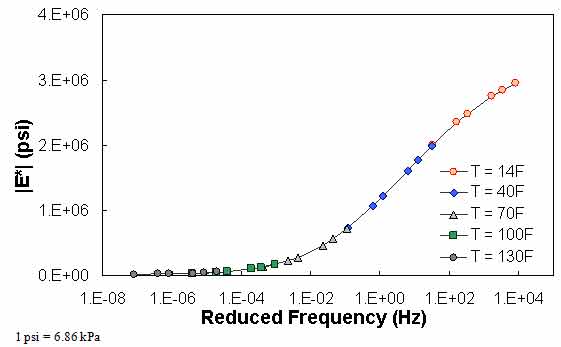
Figure 61. Graph. Example of the effect of a violation of QC #1 for MR ANN model in
semi-log scale.
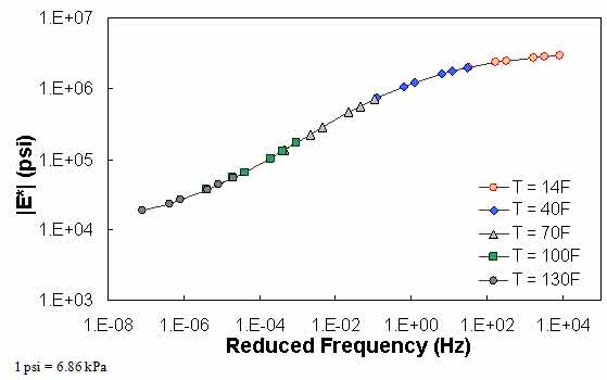
Figure 62. Graph. Example of the effect of a violation of QC #1 for MR ANN model in log-log scale.
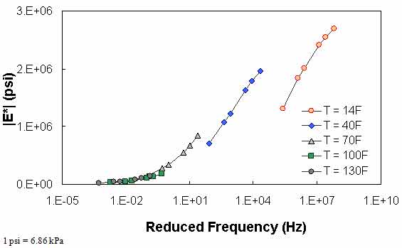
Figure 63. Graph. Example of the effect of a violation of QC #1 for VV ANN model in semi-log scale.
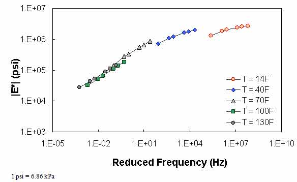
Figure 64. Graph. Example of the effect of a violation of QC #1 for VV ANN model in log-log scale.
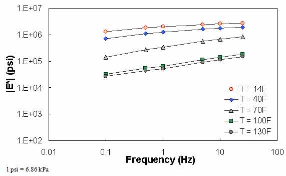
Figure 65. Graph. Example of the effect of a violation of QC #1 for VV ANN model unshifted data.
QC #2 checks the trends of |E*| as a function of temperature and frequency. It is expected that |E*| decreases as the temperature increases and the loading frequency decreases. Figure 66 through figure 68 show sample cases of a QC #2 violation. In these examples, the predicted |E*| value at 40 °F (4.4 °C) and 25 Hz is smaller than the predicted value at 40 °F (4.4 °C) and 10 Hz. Similar to QC #1, this QC check is performed line-by-line; the lines that pass receive a grade of “A,” and those that fail receive a grade of “F.”
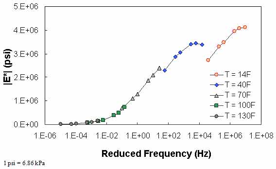
Figure 66. Graph. Example of the effect of a violation of QC #2 in semi-log scale.
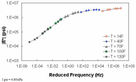
Figure 67. Graph. Example of the effect of a violation of QC #2 in log-log scale.
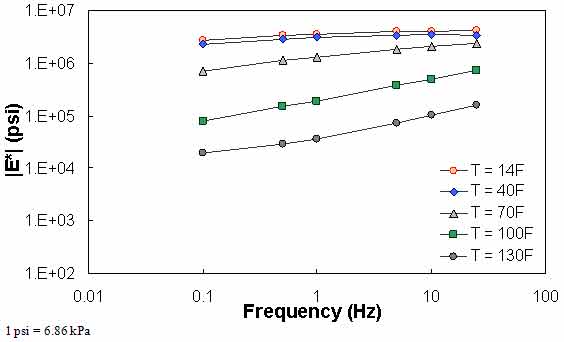
Figure 68. Graph. Example of the effect of a violation of QC #2 unshifted data.
The typical percentage of difference between 0.1 Hz at one temperature and 25 Hz at the next warmest temperature is checked using QC #3. Equation 51 states the percentage of difference and a typical value of this term based on the available data in this study. Figure 69 through figure 71 show the violation of QC #3 in one of the sections. For this particular section, a violation occurred between 40 and 70 °F (4.4 and 21.1 °C). For this sample case, at 0.1 Hz and 40 °F (4.4 °C), the modulus is equal to 1.29 x 10⁶ psi (8.85 x 10⁶ kPa). At 25 Hz and 70 °F (21.1 °C), the modulus is equal to 8.28 x 10⁵ psi (56.8 x 10⁵ kPa), which is a percentage difference of 55.4 percent.
 |
(51) |
Unlike the previous QC checks, QC #3 is performed on the basis of temperature. For example, if the percentage of difference between 14 and 40 °F (-10 and 4.4 °C) exceeds 25 percent, then all of the predictions at 14 °F (-10 °C) would receive a grade of “F.”
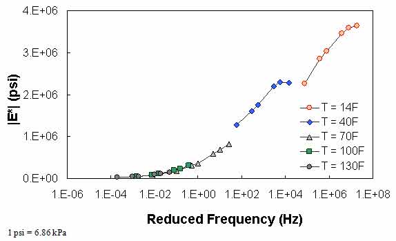
Figure 69. Graph. Example of the effect of a violation of QC #3 in semi-log scale.
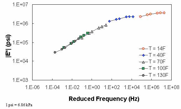
Figure 70. Graph. Example of the effect of a violation of QC #3 in log-log scale.
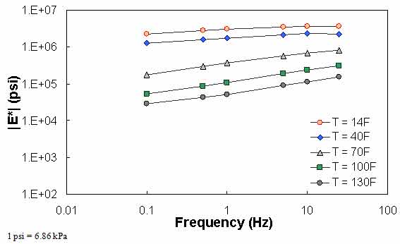
Figure 71. Graph. Example of the effect of a violation of QC #3 unshifted data.
in QC #4, the difference in |E*| values predicted between 0.1 Hz at one temperature and 0.1 Hz at the next warmest temperature is checked to see if appropriate trends with regard to temperature and modulus hold. Sample cases of QC #4 violation are shown in figure 72 through figure 74. For the data in these figures, |E*| at 0.1 Hz and 40 °F (4.4 °C) is smaller than |E*| at 0.1 Hz and 70 °F (21.1 °C). In the case shown in these figures, this situation has led to a discontinuous mastercurve because the optimization algorithm becomes confused when the modulus does not decrease as the temperature increases. Similar to QC #3, QC #4 is applied on a temperature basis.
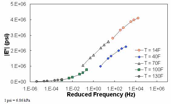
Figure 72. Graph. Example of the effect of a violation of QC #4 in semi-log scale.
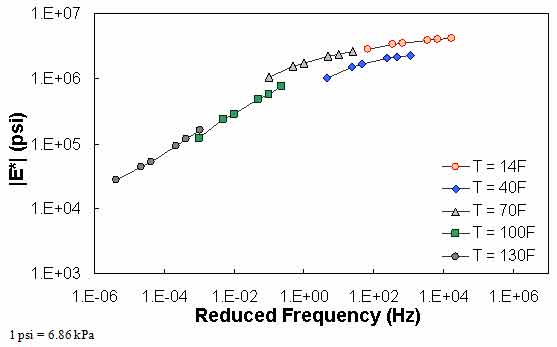
Figure 73. Graph. Example of the effect of a violation of QC #4 in log-log scale.
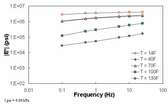
Figure 74. Graph. Example of the effect of a violation of QC #4 unshifted data.
QC #5 checks the range of shift factor values in the output predictions against typical values. This check is used to indicate potential problems with the mastercurve generation process. The limits identified and subsequently used are as follows:
The output parameters of interest from the ANNACAP software are SHIFT_FACTOR COEFFICIENT 1 (α1), SHIFT_FACTOR_COEFFICIENT 2 (α2), and SHIFT_FACTOR_COEFFICIENT 3 (α3). The shift factor is computed using equation 52 as follows:
| (52) |
Because the goal of this QC criterion is to judge the mastercurve generation process, only shift factor values at extreme temperatures need to be examined. Note that because the MR ANN model predicts the mastercurve directly, any predictions made with this model will automatically pass QC #5 without the need for calculation. When this QC is not passed, the entire section (at all temperatures) receives a grade of “F.”
Figure 75 through figure 77 show violations of QC #5. In these cases, the shift factor at 14 °F (-10 °C) is equal to 7.03. This effect results in a visual discontinuity in the mastercurve between the 14- and 40-°F (-10- and 4.4-°C) datasets.
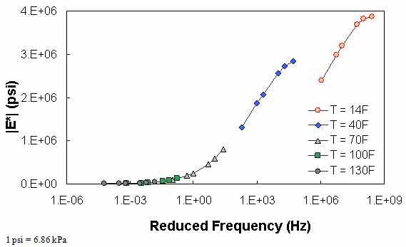
Figure 75. Graph. Example of the effect of a violation of QC #5 in semi-log scale.
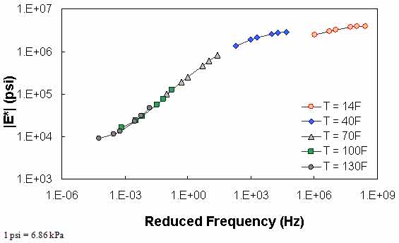
Figure 76. Graph. Example of the effect of a violation of QC #5 in log-log scale.
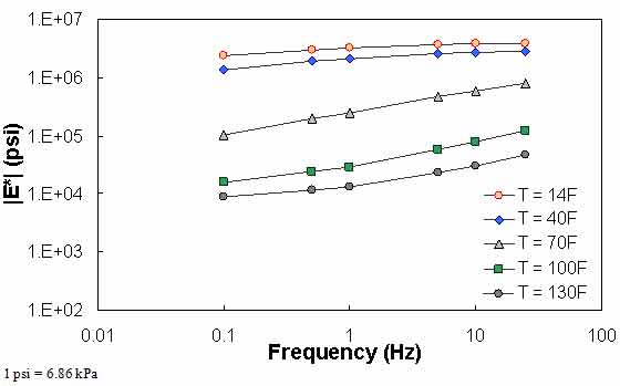
Figure 77. Graph. Example of the effect of a violation of QC #5 unshifted data.
In an earlier version of the ANN models developed for this study, some cases had inputs within the calibration input range, but the |E*| predictions obtained values of the limits of the calibration data. In some other cases, |E*| did not change with varying temperature and frequency. QC #6 was expected to be the last QC check, but after improving the ANN models, the problem no longer exists. Nevertheless, the check is performed on the data. The limiting |E*| values used to judge whether a given prediction passes this QC check are given in table 25. Like QC #1 and QC #2, this QC check is applied line-by-line.
| Model | Upper Limit (psi) | Lower Limit (psi) |
|---|---|---|
| MR ANN | N/A | N/A |
| VV ANN | 5,888,437 | 3,311.311 |
| GV ANN | 6,456,542 | 3,311.311 |
|
1 psi = 6.86 kPa |
||
Similar to QC #5, QC #7 is designed to judge the mastercurve generation process. Each time a mastercurve is generated, fitting statistics are computed. These statistics include the Se/Sy (of combined predictions), and R2. According to the draft standard for mastercurve generation using AASHTO TP-62 data, the explained variance should be greater than 0.99, and the ratio of Se/Sy should be less than 0.05.(42) When these limits are exceeded, QC #7 is triggered, and the layer fails. Because the MR ANN model predicts the mastercurve directly, any predictions made with this model will automatically pass QC #7 without the need for calculation. Equations 53–55 are used to compute the necessary statistical parameters. Whenever this QC is violated, the entire section receives a grade of “F.”
| (53) |
Where:
| 23 | = | Number of temperature/frequency combinations used minus the number of fitting parameters minus 1. |
|---|---|---|
| (log|E*|ANN)i | = | Logarithm of the modulus determined from the ANN models at a particular temperature frequency combination. |
| (log|E*|fit)i | = | Logarithm of the modulus determined from the optimized sigmoidal fit. |
 |
(54) |
Where:
| 29 | = | Number of temperature/frequency combinations used minus 1. |
|---|---|---|
| (log|E*|avg)i | = | Logarithm of the average modulus determined from the ANN models for a given layer. |
| (55) |
The NCSU researchers used a combination of the above QC factors to judge the quality of the modulus prediction for an individual modulus prediction. If QCs #1, #3, #4, and #6 all pass, then the section receives a grade of “A.” If QC #1 fails but QCs #3, #4, and #6 all pass, then the modulus receives a grade of “C,” which means the predicted moduli are questionable. Otherwise, the modulus receives a grade of “F.”
QCs #5 and #7 are used to judge the quality of the calibrated mastercurve and shift factor function. When both QCs pass, the section receives a grade of “A,” but when both fail, the section receives a grade of “F.” If one passes and one fails, then the mastercurve and shift factor function values are questionable, and the section receives a grade of “C.”
The LTPP database contains information for a total of 1,806 layers that meet the criteria described in section 3.4 of this report. These layers have binder data available at a combination of different aging conditions including unaged or original-, RTFO-, PAV-, or field-aged. In the field-aged data, 2,223 records are available because some layers' properties may have been measured at different dates. The total resulting number of records is 7,641. Using the combined ANN models and requisite QC checks, modulus values were predicted for 363 records/layers in the original-aged level, 469 records/layers in the RTFO-aged level, 1 record/layer in the PAV level, and 503 records in the field-aged level. These numbers translate to predictions for 17.5 percent of the total number of records available. However, these records are distributed in such a way that a higher percentage of the layers have some sort of valid prediction. Of the 1,806 layers in the database, 1,010, or 56 percent, have a modulus prediction at some aging condition. Of these 1,010 layers, 615, or 34 percent of the total 1,806 layers, have completely reasonable predictions (i.e., an “A” grade), and 89, or 4.9 percent of the total 1,806 layers, have unreasonable predictions (i.e., an “F” grade). The remaining 306 layers (17 percent of the 1,806 layers) have questionable predictions (i.e., a “C” grade). Thus, the total percentage of layers with a completely valid or questionable prediction is 51 percent. Table 26 shows the summarized statistics of the population effort. Although it cannot be interpreted directly from this table, the majority of the valid records were populated using the MR ANN model followed next by the VV-grade ANN model and the VV ANN model.
| Populated LTPP data | Aging Condition | Total | ||||
|---|---|---|---|---|---|---|
| Original | RTFO | PAV | Field | |||
| Number of records | 1,806 | 1,806 | 1,806 | 2,223 | 7,641 | |
| Number of populated records | 363 | 469 | 1 | 503 | 1,336 | |
| Number of records by contractor individual judgment grade | Grade A | 147 | 252 | 0 | 465 | 864 |
| Grade C | 0 | 1 | 1 | 38 | 40 | |
| Grade F | 216 | 216 | 0 | 0 | 432 | |
| Number of records by contractor mastercurve judgment grade | Grade A | 44 | 142 | 0 | 0 | 186 |
| Grade C | 211 | 237 | 0 | 503 | 951 | |
| Grade F | 108 | 90 | 1 | 0 | 199 | |
| Populated records using MR | 5 | 0 | 0 | 503 | 508 | |
| Populated records using VV | 358 | 59 | 0 | 0 | 417 | |
| Populated records using GV | 0 | 0 | 1 | 0 | 1 | |
| Populated records using GV-PAR | 0 | 2 | 0 | 0 | 2 | |
| Populated records using VV-grade | 0 | 408 | 0 | 0 | 408 | |
| Number of populated layers | 1,010 | |||||
| Number of layers with valid and questionable predictions | 921 | |||||
| Number of layers with fully valid predictions | 615 | |||||
| Number of layers with failed predictions | 89 | |||||
As a result of this project, nine tables were included in the LTPP database to document the inputs used in the dynamic modulus models as well as resultant predictions.(20) The tables were added to the materials testing module (i.e., TST) of the LTPP database. Each table is described below. It should be noted that inputs from the LTPP database as well as outputs from the models are in units that are consistent with popular convention, but both SI and English units are used in the tables.
| Field Name | Field Description |
|---|---|
| ESTAR_LINK | Generic key for linking ESTAR data |
| STATE_CODE | Numerical code for State or province. U.S. codes are consistent with Federal Information Processing Standards |
| SHRP_ID | Test section identification number assigned by LTPP program. Must be combined with STATE_CODE to be unique |
| LAYER_NO | Unique sequential number assigned to pavement layers starting with layer 1 as the deepest layer (subgrade) |
| PROJECT_ID | The four-character identifier for the SPS project used to identify elements of information which are common to all sections in that project |
| PROJECT_LAYER_CODE | Sequential alphabetic code assigned to identify group project-wide layers |
| PREDICTIVE_MODEL | Code indicating the predictive model used to generate ESTAR estimates |
| CONSTRUCTION_DATE | Construction date of the layer |
| SAMPLE_TYPE_ESTAR | Code indicating the aging condition of the samples used for inputs into the ESTAR predictive models |
| SAMPLE_DATE | Sampling date if field-aged |
| SAMPLE_AGE | Sample age if field-aged |
| RECORD_STATUS | Code indicating the general quality of the data as outlined, based on the level of QC checks described in the Database User Reference Guide(10) |
| Field Name | Field Description |
|---|---|
| ESTAR_LINK | Generic key for linking ESTAR data |
| TEMPERATURE | Temperature of modulus prediction |
| FREQUENCY | Frequency of modulus prediction |
| ESTAR | Predicted dynamic modulus |
| RECORD_STATUS | Code indicating the general quality of the data as outlined, based on the level of QC checks described in the Database User Reference Guide(10) |
| Field Name | Field Description |
|---|---|
| ESTAR_LINK | Generic key for linking ESTAR data |
| SIGMOIDAL_COEFF_1 | Sigmoidal fitting function coefficient delta |
| SIGMOIDAL_COEFF_2 | Sigmoidal fitting function coefficient alpha |
| SIGMOIDAL_COEFF_3 | Sigmoidal fitting function coefficient beta |
| SIGMOIDAL_COEFF_4 | Sigmoidal fitting function coefficient gamma |
| SHIFT_FACTOR_COEFF_1 | Shift factor fitting function coefficient alpha 1 |
| SHIFT_FACTOR_COEFF_2 | Shift factor fitting function coefficient alpha 2 |
| SHIFT_FACTOR_COEFF_3 | Shift factor fitting function coefficient alpha 3 |
| MASTERCURVE_QUALITY | Code indicating the general quality of the mastercurve generation process. Pass if explained variance is greater than 0.99 and ratio of standard error to standard deviation is less than 0.05 |
| RECORD_STATUS | Code indicating the general quality of the data as outlined based on the level of QC checks described in the Database User Reference Guide(10) |
| Field Name | Field Description |
|---|---|
| ESTAR_LINK | Generic key for linking ESTAR data |
| TEMPERATURE | Temperature of modulus prediction |
| FREQUENCY | Frequency of modulus prediction |
| GSTAR | Binder shear modulus used for G* ANN model |
| RECORD_STATUS | Code indicating the general quality of the data as outlined based on the level of QC checks described in the Database User Reference Guide(10) |
| Field Name | Field Description |
|---|---|
| ESTAR_LINK | Generic key for linking ESTAR data. |
| CAM_COEFF_1 | CAM fitting function coefficient Gg |
| CAM_COEFF_2 | CAM fitting function coefficient wc |
| CAM_COEFF_3 | CAM fitting function coefficient k |
| CAM_COEFF_4 | CAM fitting function coefficient me |
| RECORD_STATUS | Code indicating the general quality of the data as outlined based on the level of QC checks described in the Database User Reference Guide(10) |
| Field Name | Field Description |
|---|---|
| ESTAR_LINK | Generic key for linking ESTAR data |
| VMA | Voids in mineral aggregate as a percent of total volume |
| VFA | Voids filled with asphalt as a percent of VMA |
| RECORD_STATUS | Code indicating the general quality of the data as outlined, based on the level of QC checks described in the Database User Reference Guide(10) |
| Field Name | Field Description |
|---|---|
| ESTAR_LINK | Generic key for linking ESTAR data |
| TEMPERATURE | Temperature of modulus prediction |
| VISCOSITY | Voids filled with asphalt as a percent of VMA |
| RECORD_STATUS | Code indicating the general quality of the data as outlined, based on the level of QC checks described in the Database User Reference Guide(10) |
| Field Name | Field Description |
|---|---|
| ESTAR_LINK | Generic key for linking ESTAR data |
| VISC_A | Viscosity model intercept |
| VISC_VTS | Viscosity model slope |
| RECORD_STATUS | Code indicating the general quality of the data as outlined, based on the level of QC checks described in the Database User Reference Guide(10) |
| Field Name | Field Description |
|---|---|
| ESTAR_LINK | Generic key for linking ESTAR data |
| MR_5C | Resilient modulus at 5 °C |
| MR_25C | Resilient modulus at 25 °C |
| MR_40C | Resilient modulus at 40 °C |
| RECORD_STATUS | Code indicating the general quality of the data asoutlined, based on the level of QC checks described in the Database UserReference Guide(10) |
|
°C = (°F−32)/1.8 |
|
QC checks were developed to be applied to the LTPP database. These checks include many of the internal checks developed as part of this study as well as additional checks deemed appropriate. As such, the data available in the LTPP database have been subjected to both the research team's internal QC checks and the LTPP database QC checks. Figure 78 shows the ANN models and their appropriate input and output tables.
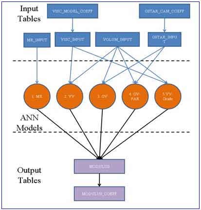
Figure 78. Illustration. ANN models and their appropriate input and output tables.

