U.S. Department of Transportation
Federal Highway Administration
1200 New Jersey Avenue, SE
Washington, DC 20590
202-366-4000
Federal Highway Administration Research and Technology
Coordinating, Developing, and Delivering Highway Transportation Innovations
| REPORT |
| This report is an archived publication and may contain dated technical, contact, and link information |
|
| Publication Number: FHWA-HRT-10-035 Date: September 2011 |
Publication Number: FHWA-HRT-10-035 Date: September 2011 |
Three ANN models have been developed for populating the LTPP database sections. These models are differentiated by the following primary input parameters: (1) the MR model uses the resilient modulus, (2) the VV model uses the binder viscosity, and (3) the |G*|-based (GV) model uses the binder shear modulus. The subsequent sections provide a description of each model along with the final verification plots and statistics. The models in this chapter use normalized inputs, whereas those discussed in the previous section use nonnormalized inputs.
The term normalizing a vector often refers to changing the magnitude of an element by dividing it by a norm of the vector. For neural networks, this definition often means changing the scale of a vector by the minimum value and the range of the vector so that all the components are between 0 and 1 or 1 and -1. Linear and uniform normalizations are the common methods used for this purpose. In some cases, such as lab- and field-measured data used to develop the ANN models in this study, linear normalization seems to be more meaningful when no specific distributions of the data are known or present. In addition to normal distribution, a Gaussian normalization (based on the mean and standard deviation of the data for each parameter) could be performed. In some cases, these statistics could be used to get rid of outliers (e.g., data points outside of the three standard deviations). Although such types of nonlinear normalization and related procedures may be useful in some applications (e.g., when the measurement range is meant to be normally distributed or distributed with some statistical uniformity), for the type of engineering applications where the data represent different conditions, it is not possible to find a statistical distribution of those input values. For example, if temperature is an input and different datasets represent different discrete values/ranges, then it is not useful to find a mean temperature value and its standard deviation to normalize the data. In this study, the linear model was adopted because of its simplicity. After applying this normalization (scaling) scheme to the data and developing the ANN models, it was found that the predictions were acceptable, and there was no further investigation into the need of nonlinear normalization. This issue is one that possibly warrants future study.
The decision to utilize normalized input-based ANN models was not finalized at the time of the study presented in the previous chapter. After deciding to use normalized input-based ANN models, the pilot analysis was not redone because the normalization only improved the predictability and thus did not change the final conclusions of the pilot study. Based on these fitting statistics and on engineering judgment, the models were ranked to develop a decision tree so that a user can determine which ANN model is best suited to a specific set of input parameters.
Due to differences in the required inputs for each model, different subsets of the entire database were used in training and verification. The total number of points used for each model, along with a summary of the required input parameters, is provided in table 21. Of the total available points for each model, 90 percent were randomly selected for the purpose of training the networks, and 10 percent were used for verification. The Witczak database was used for calibrating the VV ANN model, except that the data at the temperatures equal to or less than 32 ° F (0 °C) were not used because of unacceptably high |E*| values. It should be mentioned that the GV and |G*|-based model using inconsistent aged binder data of PAV- and RTFO-aging conditions (GV-PAR) models, like the VV and viscosity-based model using specification grade of the asphalt binder (VV-grade) models, represent the same trained network, but they are identified by different terms due to the binder values used in each case. In the GV-PAR model, the binder values are based on two aging conditions, PAV and RTFO. In the VV-grade model, the values of A and VTS are chosen, as recommended in MEPDG, based on the specification grade of the asphalt binder. Sections using this model have less than two viscosity measurements, but the VMA, VFA, and binder grade values are available. Descriptions of the binder analysis necessary for using these models are given in appendices A and B.
All of the ANN models developed herein contain a mapping ANN architecture and are based on supervised learning. In the developed network, the learning method used is a feed forward back propagation, and the sigmoidal function is the transfer function. The three-layer network with two hidden layers was selected as the best configuration. The number of nodes in each layer differs according to the selected model (see table 21). These node numbers were determined after a systematic study of each model. In each case, the network follows the same basic structure that is schematically illustrated in figure 41. A more formal mathematical representation for each of these models is given in appendix D.
| ANN Model | Parameters Used to Train ANN Models | Number of Data Points | Number of Nodes | ||||||
|---|---|---|---|---|---|---|---|---|---|
| MR at 5, 25, and 40 °C (MPa) | Shift Factor(α1, α2, α3) | fR (Hz) | Viscosity (109 P) | VMA (Percent) | VFA (Percent) | |G*| (psi) | |||
| MR | ✓ | ✓ | 11,730 | 12 | |||||
| VV | ✓ | ✓ | ✓ | ✓ | 14,682 | 14 | |||
| GV | ✓ | ✓ | ✓ | 12,907 | 12 | ||||
| GV-PAR | ✓ | ✓ | ✓ | 12,907 | 12 | ||||
| VV-grade | ✓ | ✓ | ✓ | ✓ | 14,682 | 14 | |||
|
°C = (°F−32)/1.8 |
|||||||||
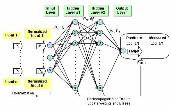
Figure 41. Illustration. Network structure used for training the ANN models.
The 1993 AASHTO Guide for Design of Pavement Structures employs MR as the material property representing the stiffness characteristics of layer materials. (27) MR is defined as the ratio between applied stress (σa) and recoverable strain (εr) as follows:
| (19) |
Several testing standards have been developed for the determination of MR of AC using the indirect tensile (IDT) test method (American Society for Testing and Materials (ASTM) D4123-82, NCHRP 1-28, State Highway Research Program (SHRP) P-07, and NCHRP 1-28A). (See references 28–31.) In light of these facts, the LTPP database has stored MR as the primary measured mixture stiffness term for many of the layers. Due to the industry's transition from MR to |E*|, a significant amount of MR data that have been collected in State highway agencies may become obsolete unless the MR values can be converted to |E*| values. The NCSU research team successfully developed a method to make this conversion using an ANN-based methodology to predict the |E*| values at multiple temperatures and frequencies when only the MR values at three temperatures are available.
The difficulty in performing this conversion stems from the fact that MR provides a snapshot of the material behavior under one loading history (i.e., 0.1-s haversine loading followed by a 0.9-s rest period) at different testing temperatures (normally three temperatures at 41, 77, and 104 °F (5, 25, and 40 °C)). Zhang explored the possibility of characterizing the viscoelastic properties obtained from MR tests using Fourier analysis.(32) It was concluded that this type of analysis is impractical due to the difficulty in solving a large number of variables and the limited range of results, which provided little information other than MR data. Another challenge is that Fourier analysis requires a loading and deformation history in order to fit, which most databases do not contain. Because an analytical method is not feasible, any attempt to predict |E*| from MR is, at best, empirical in nature.
One difficulty in any empirical model is acquiring a database large enough to represent the range of possible inputs. Because a large database containing both MR and |E*| does not exist, a theoretical approach has been developed based on LVE principles. The resulting forward model is used along with the mixtures in the Witczak database to develop the ANN model training database.
Developing a database with |E*| and MR values can be a time-consuming task if the properties are measured in the laboratory, especially for a database comprehensive enough to encompass a large range of mixture variables such as binders, gradations, NMSA, VMA, VFA, air voids, etc. The proposed method was to use a comprehensive |E*| database and populate the database with MR values by using LVE principles.
MR can be calculated by several different methods, including ASTM D4123-82, NCHRP 1-28 method, the SHRP P07 protocol, AASHTO TP31-96 standard, or the Roque and Buttlar equation 17, which accounts for the bulging effects of the specimen. (See references 28, 29, 30, 33, and 34.) The NCHRP 1-28 elastic solutions are used in this report.(29) The equations for calculating MR and Poisson's ratio are as follows:
| (20) |
| (21) |
Where:
| MR | = | Resilient modulus (MPa). |
|---|---|---|
| ν | = | Poisson's ratio. |
| P | = | Applied load (N). |
| U | = | Recoverable horizontal displacement (m). |
| V | = | Recoverable vertical displacement (m). |
| k1, k2, k3, k4 | = | Constants. |
Equations 20 and 21 can be combined to yield the following relationship:
 |
(22) |
These equations are based on the linear elastic solutions developed by Hondros after accounting for the nonuniform stress and strain distributions in the IDT specimen (see figure 42).(35) The constants in equations 20 and 21 are listed in table 22. Note that these constants are different from the constants for |E*| because the coefficients for MR are derived using linear elastic theory, whereas those for |E*| are derived using LVE theory.
| IDT |E*| | β1 | β2 | ϒ1 | ϒ2 |
| -0.0134 | -0.0042 | 0.0037 | 0.0116 | |
| MR | k3 | k4 | k1 | k2 |
| -0.00067 | 0.000209 | -0.00018 | 0.000578 |
Figure 42. Illustration. Stress distribution in the IDT specimen subjected to a strip load.
For linear elastic materials, the stress-strain relationship is represented by the generalized Hooke's law. It is assumed that the rectangular coordinate of x1 is in the horizontal direction, x2 is in the vertical direction, and x3 is in the depth direction of the IDT specimen. Two strains that are of interest are ε11 and ε22. According to the generalized Hooke's law, these two strains are related to stresses as follows:
| (23) |
| (24) |
Where:
| E | = | Young's modulus. |
|---|---|---|
| D | = | Compliance. |
Application of the elastic-viscoelastic correspondence principle to these linear elastic solutions results in the following LVE stress-strain relationships:
 |
(25) |
 |
(26) |
The Hondros equations used to calculate the resulting stresses in the horizontal and vertical directions are as follows:
| (27) |
| (28) |
| (29) |
 |
(30) |
Where:
| R | = | Radius of specimen (m). |
|---|---|---|
| x | = | Horizontal distance from center of specimen (m). |
| a | = | Radial angle (radians). |
Combining equation 27 through equation 30 results in the following expressions for the horizontal and vertical strains:
| (31) |
| (32) |
The displacements at the gauge length can be calculated by integrating the nonuniform strains in equations 31 and 32 along the gauge length (i.e., -l to +l) as follows:
| (33) |
| (34) |
or
| (35) |
 |
(36) |
For the gauge length of 2.0 inches (50.8 mm), equations 35 and 36 reduce to the following:
 |
(37) |
| (38) |
Where the values of β1, β2, ϒ1, and ϒ2 are shown in table 22. Equations 37 and 38 require two time-dependent material properties (i.e., creep compliance and Poisson's ratio). It has been proven that the creep compliance of AC can be predicted from |E*| using theoretical relationships.(36) In this study, the following approach |E*|mastercurve to the creep compliance.
The complex modulus, E*, is represented in equation 39 as follows:
 |
(39) |
Where:
| E' | = | Storage modulus = |E*| cosine . |
|---|---|---|
| E" | = | Loss modulus = |E*| sine . |
| ø | = | Phase angle. |
The storage modulus, E', can be represented in terms of a Prony series in equation 40 as follows:
 |
(40) |
Where:
| E∞ | = | Elastic modulus (MPa). |
|---|---|---|
| ωr | = | Angular reduced frequency. |
| Ei | = | Modulus of the ith Maxwell element. |
| ρi | = | Relaxation time of the ith Maxwell element. |
An exact conversion to D(t) can be obtained by solving the following equations:
| (41) |
| (42) |
| (43) |
Where:
| Akj | = | Matrix element in the kth row and jth column of matrix A. |
|---|---|---|
| Bk | = | Vector element in the kth row of vector B. |
| E∞ | = | Equilibrium modulus (MPa). |
| Ei | = | Modulus of the ith Maxwell element. |
| ρi | = | Relaxation time of the ith Maxwell element determined a priori. |
| tj | = | Retardation time of the jth Voigt element determined a priori. |
| tk | = | Time of interest. |
| m | = | Number of Prony coefficients. |
By solving for compliance of column j of matrix A (Dj), the Prony series representation for D(t) can be determined. Equation 42 does not show a solution for ρi = τj because the error increases when such a case exists.(36,37)
The second time-dependent material property in equation 37 is Poisson's ratio. The time-dependent nature of Poisson's ratio has been reported.(37) Poisson's ratio values for the S12.5C mixture are shown in figure 43 against the reduced time to show a typical trend.
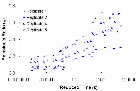
Figure 43. Graph. Poisson's ratio versus reduced time for S12.5C.
The Poisson's ratio values are calculated from equation 21 using the data from the IDT |E*| test. As can be seen in figure 43, a large sample-to-sample variability is evident in Poisson's ratio values. Another problem with Poisson's ratio is that equation 25 is difficult to solve because two time-dependent properties are inherent in the equation. If Poisson's ratio in equations 25 and 26 is assumed to be constant, the two equations reduce to the following:
 |
(44) |
 |
(45) |
In figure 43, the measured Poisson's ratio exceeds the theoretical limits of zero to 0.5. A high Poisson's ratio occurs at large reduced times when the temperature is high and/or the loading time is long. Some Poisson's ratios are higher than 0.5, indicating that damage has occurred in the specimen.(28,38) The biggest challenge in determining Poisson's ratio in the IDT test is to induce a large enough horizontal displacement to overcome the electronic noise in the testing system without causing damage in the specimen. Mirza et al. provide a method to evaluate the quality of the data using a deflection ratio.(39)
The effect on MR when a constant Poisson's ratio is assumed is evaluated by using three Poisson's ratios at each temperature of each mixture and calculating the percentage of difference in the predicted MR values. The Poisson's ratio values used in this comparison are 0.15, 0.2, and 0.25 for 41 °F (5 °C); 0.25, 0.3, and 0.35 for 77 °F (25 °C); and 0.4, 0.45, and 0.5 for 104 °F (40 °C). It was found that the difference in MR values is negligible when Poisson's ratio, which is used to predict the displacements, is used to calculate MR. A more indepth analysis of equations 20 and 37 along with the geometry coefficients in these equations, which are shown in table 22 (i.e., k1, k2, 1, and 2), reveals that the effect of change in Poisson's ratio on the term (k1-k2n) in the numerator of equation 20 is about the same as that on the horizontal displacement calculated from equation 37, which appears in the denominator of equation 20. Therefore, it is concluded that the effect of Poisson's ratio on MR calculation is minimal. Vinson draws a similar conclusion that a Poisson's ratio of 0.15 to 0.45 does not affect MR much based on a theoretical finite-element analysis.(40,28) For the remainder of this report, equation 44 is used, with constant Poisson's ratios of 0.2, 0.35, and 0.45 for 41 °F (5 °C), 77 °F (25 °C), and 104 °F (40 °C), respectively.
Because the numerical integration of equation 44 requires calculating all the previous time steps to arrive at the current time step, calculation times can grow exponentially.(41) To reduce the calculation time, the state variable approach described in equation 46 through equation 48 is used in this study.
| (46) |
Where:
| (47) |
| (48) |
Figure 44 through figure 47 show the results of predicted versus measured values using a LOE graph. For both mixtures, the predicted and measured MR values are in good agreement, suggesting that the proposed approach based on the theory of linear viscoelasticity using the IDT |E*| can provide a reasonable estimate of MR of AC.
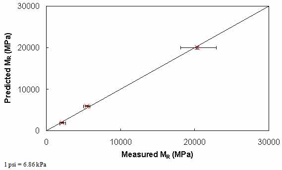
Figure 44. Graph. Comparison of predicted and measured MR values for S12.5C mixture.
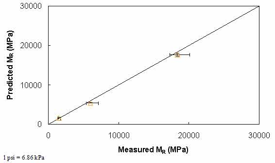
Figure 45. Graph. Comparison of predicted and measured MR values for S12.5CM mixture.
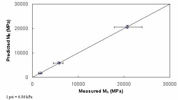
Figure 46. Graph. Comparison of predicted and measured MR values for S12.5FE mixture.
Figure 47. Graph. Comparison of predicted and measured MR values for B25.0C mixture.
The characterization and verification results of the MR ANN model are shown in figure 48 through figure 51. In figure 49, the results of characterization are shown in logarithmic space, and the model displays excellent fitting statistics with a high R2 = 0.98 (0.90 in arithmetic space) and a low Se/Sy = 0.15 (0.32 in arithmetic space). The verification plots are shown in figure 50 and figure 51, and the model is found to predict the moduli values with statistics similar to those from the calibration dataset.
Figure 48. Graph. MR ANN model using 90 percent of randomly selected data as a training set in arithmetic scale.
Figure 49. Graph. MR ANN model using 90 percent of randomly selected data as a training set in logarithmic scale.
Figure 50. Graph. MR ANN model using 10 percent of randomly selected data as a verification set in arithmetic scale.
Figure 51. Graph. MR ANN model using 10 percent of randomly selected data as a verification set in logarithmic scale.
The characterization and verification results of the VV ANN model are shown in figure 52 through figure 55 in a manner similar to that shown for the MR ANN model. Like the MR ANN model, the VV model shows good fitting statistics with a high R2 = 0.95 (0.93 in arithmetic space) and a low Se/Sy = 0.23 (0.26 in arithmetic space). The verification plots are shown in figure 54 and figure 55. Although the verification statistics are not as favorable as those found for the MR— ANN model, they are still better overall than those of the existing closed-form solutions.
Figure 52. Graph. VV ANN model using 90 percent of randomly selected data as a training set in arithmetic scale.
Figure 53. Graph. VV ANN model using 90 percent of randomly selected data as a training set in logarithmic scale.
Figure 54. Graph. VV ANN model using 10 percent of randomly selected data as a verification set in arithmetic scale.
Figure 55. Graph. VV ANN model using 10 percent of randomly selected data as a verification set in logarithmic scale.
The characterization and verification results of the GV ANN model are shown in figure 56 through figure 59. The calibration dataset for this model shows similar or slightly better fitting statistics than the VV ANN model, with an R2 = 0.96 (0.90 in arithmetic space) and a Se/Sy = 0.19 (0.32 in arithmetic space). The verification plots are shown in figure 58 and figure 59, and the model predictions agree favorably with the measured moduli. Care must be taken when visually comparing the predictability of the VV ANN and GV ANN models because each uses a different number of datapoints for calibration and verification (see table 21).
Figure 56. Graph. GV ANN model using 90 percent of randomly selected data as a training set in arithmetic scale.
Figure 57. Graph. GV ANN model using 90 percent of randomly selected data as a training set in logarithmic scale.
Figure 58. Graph. GV ANN model using 10 percent of randomly selected data as a verification set in arithmetic scale.
Figure 59. Graph. GV ANN model using 10 percent of randomly selected data as a verification set in logarithmic scale.
Through the course of this study, some effort was made to develop ANN models with gravimetric (as opposed to volumetric) input variables. Ultimately, these models were not fully developed nor were they used in the modeling efforts because, after a preliminary review, it was determined that such models would not be useful. Although it is true that some layers contained gravimetric-based effective asphalt contents, these sections also contained enough information to allow the volumetric properties VMA and VFA to be computed. The most common relationship for the three key volumetric properties is shown in equation 49 as follows:
| (49) |
For statistical validity, the expected error for each of the three main ANN models has been assessed using the following error function:
 |
(50) |
A probability distribution function for the error was computed for each model by using the verification dataset for the respective model. These datasets are shown in figure 50 and figure 51 for MR ANN, figure 54 and figure 55 for VV ANN, and figure 58 and figure 59 for GV ANN. The distribution function is shown for each model, including the previously discussed closed-form models presented in table 23. The distribution of each error function is approximately normal and, as such, the error values that encompass a 95 percent reliability interval for the percentage of error in each model can be readily computed.
Because the number of data points used to verify each model is so large (see the last row in table 23), the distribution is assumed normal, and a z-score of 1.96 is used to compute the reliability ranges. Sy is computed after compiling the percent error values for each prediction of the respective model. After rounding slightly for convenience, the suggested reliability range for each ANN model is as follows:
It is also found from table 23 that when the closed-form solutions are applied to a completely independent dataset, each solution yields a substantial number of predictions with errors exceeding -105 percent. The dataset used to compute these statistics is completely independent of the data used in calibrating any of these closed-form solutions. It also includes a mixture of AMPT and TP-62 measured moduli.(8) The high number of large negative error observations suggests a bias towards over-prediction of the |E*| values with each model. The bias in predictions can be clearly observed by examining figure 8 for the modified Witczak model and figure 10 for the Hirsch model. A comparison of figure 7 and figure 9 shows a tendency of the Hirsch model to underpredict |E*| at higher modulus values more so than the modified Witczak model. This trend is also captured in table 23, where the error distribution for the Hirsch model is skewed towards positive values. As a result of the existence of these prediction errors, the reliability ranges for the closed-form solutions are much larger than the ranges observed for the ANN models as follows:
| Percentage Error Range | ANN Model (Percentage Within Range) | |||||
|---|---|---|---|---|---|---|
| MR | VV | GV | Original Witczak | Modified Witczak | Hirsch | |
| < -105 | 0.75 | 2.31 | 0.49 | 22.04 | 31.12 | 10.25 |
| -105 to -90 | 0.32 | 0.86 | 0.77 | 2.86 | 5.11 | 2.65 |
| -90 to -75 | 0.43 | 1.91 | 1.05 | 3.15 | 8.43 | 3.14 |
| -75 to -60 | 0.21 | 2.44 | 2.02 | 3.72 | 8.97 | 4.46 |
| -60 to -45 | 0.53 | 4.75 | 3.42 | 7.06 | 10.49 | 5.86 |
| -45 to -30 | 5.98 | 7.59 | 8.02 | 8.30 | 11.39 | 8.58 |
| -30 to -15 | 15.06 | 14.32 | 16.11 | 9.83 | 9.24 | 12.34 |
| -15 to 0 | 24.89 | 17.56 | 21.34 | 10.11 | 7.89 | 14.57 |
| 0 to 15 | 28.53 | 19.14 | 21.48 | 12.02 | 4.48 | 13.81 |
| 15 to 30 | 19.02 | 15.12 | 15.69 | 13.65 | 2.06 | 10.11 |
| 30 to 45 | 3.74 | 8.65 | 6.28 | 6.20 | 0.54 | 7.67 |
| 45 to 60 | 0.32 | 4.16 | 2.58 | 1.05 | 0.27 | 4.81 |
| 60 to 75 | 0.21 | 1.06 | 0.63 | 0.00 | 0.00 | 1.39 |
| 75 to 90 | 0.00 | 0.13 | 0.14 | 0.00 | 0.00 | 0.35 |
| > 105 | 0.00 | 0.00 | 0.00 | 0.00 | 0.00 | 0.00 |
| Number of data points used | 936 | 1,515 | 1,434 | 1,048 | 1,115 | 1,434 |

