U.S. Department of Transportation
Federal Highway Administration
1200 New Jersey Avenue, SE
Washington, DC 20590
202-366-4000
Federal Highway Administration Research and Technology
Coordinating, Developing, and Delivering Highway Transportation Innovations
| REPORT |
| This report is an archived publication and may contain dated technical, contact, and link information |
|
| Publication Number: FHWA-HRT-10-035 Date: September 2011 |
Publication Number: FHWA-HRT-10-035 Date: September 2011 |
ANNs are used to solve problems in the asphalt pavement field with the primary application being the backcalculation of pavement layer moduli from falling weight deflectometer measurements.(21–23) This method has also been applied successfully to assess the roughness progression in flexible pavements and to analyze the surface wave data obtained from the nondestructive testing of asphalt pavements.(24,25) An often cited drawback of these approaches is their inability to extrapolate when a situation arises that is beyond that used to train the ANNs. To overcome this shortcoming, it is important that the dataset used to train the ANNs covers the entire range of conditions expected to be encountered during use. The objective of this study is to show that ANN modeling techniques can be applied to predict |E*| values of AC to a higher degree of accuracy than currently available models using the same input parameters.
A preliminary study was conducted to determine the feasibility and predictability of the ANN modeling technique relative to the existing models. This feasibility study was first conducted based on |G*| because more closed-form models exist that use this parameter as their primary input parameter. The ANN models used in this preliminary study are not the final models suggested by the research team, but they are similar in form and validation. To ensure full coverage of the expected conditions, the most recent Witczak database with available measured |G*| data and a portion of the dataset obtained at NCSU with support from the NCDOT were utilized as the TP-62 training database. Also, appropriate portions of the FHWA mobile trailer database and the WRI database (from the Kansas and Nevada sites) were considered the AMPT training database. A combination of the AMPT and TP-62 databases has been used to train the network after investigations, which are summarized in appendix C of this report.
The ANN model developed herein contains a mapping ANN architecture and is based on supervised learning. In the developed network, the learning method is a feed forward back propagation, which is one of the best known types of ANN. The sigmoidal function was chosen as the transfer function. The three-layer network was selected as the best network configuration. The first two layers consist of 12–14 nodes based on the different cases studied for the development of the models.
To evaluate the goodness of fit in arithmetic scale, |E*| is considered to be the dependent variable, and the error is given as follows:
| (16) |
Sy is defined as the standard deviation of the measured |E*| values. To evaluate the goodness of fit in logarithmic scale, the dependent variable is the log (|E*|), and the error is as follows:
| (17) |
Sy is defined as the standard deviation of the measured log (|E*|) values. The standard error is defined as follows:
 |
(18) |
Where:
| n | = | Number of observations. |
|---|
A literature review of current versions of the modified Witczak and Hirsch models showed that these two models have high goodness-of-fit statistics for their original training databases of 7,400 and 206 data points, respectively. (See references 11, 5, 12, 6, 7, and 13.) The literature purports high correlation coefficients and small errors of R2 = 0.80 and Se/Sy = 0.45 in arithmetic scale, R2 = 0.90 and Se/Sy = 0.32 in logarithmic scale for the modified Witczak model, and R2 = 0.98 in logarithmic scale for the Hirsch model. The developers of the Hirsch model report only the logarithmic-based R2 value.
These results demonstrate that the goodness-of-fit for each model is dependent on the number of observations or the width of the range of the different variables considered in the development of each model. The deterioration of the statistical parameters when these models are applied to some expanded and independent databases is not entirely unexpected given the nature of regression models. Additional insight is gained by examining line-of-equality (LOE) plots for each of the models in both arithmetic and logarithmic scales.
In this section, the existing models (including the modified Witczak, Hirsch, and Al-Khateeb models) are evaluated along with the two ANNs using the verification databases shown in figure 7 through figure 16. Also, figure 17 through figure 28 show predictions of the |E*| values from the verification databases using the different models. The first observation is that the Al-Khateeb model exhibits a significant bias (i.e., a power trend between the predicted |E*| and the measured |E*| values) in all the predictions. This finding is not entirely unexpected given the limited database used in calibrating the model. However, due to the bias relative to the other two existing models, it was decided that this model would be eliminated from consideration in any future analysis. It should be noted that the scales in figure 7 through figure 28 vary to provide the greatest clarity in the data.
The Hirsch model behaves in a reasonable fashion, although it exhibits undesirable behavior at low |E*| values in the LOE graphs shown in figure 9 and figure 10. When the prediction is good, the expectation is that a group of data points following the LOE with an oval shape in the LOE graph would be seen. However, the Hirsch predictions shown in figure 9 and figure 10 exhibit a horizontal pattern amplified in the bottom left side of the log-log LOE graph. This undesirable pattern in the Hirsch model predictions iHirHiris related to the insensitivity of the model and its inability to distinguish the performance differences among different mixtures for a given set of environmental and other conditions.(26) This issue is discussed later in this section.
The developers of the Hirsch model note that during initial development, substantial errors occurred when predictions were made at extremely high and low modulus values. The authors of the model attempted to correct this issue in subsequent efforts by expanding the calibration database to include 15.8 and 129.2 °F (-9 and 54 °C) data.(6) However, it is unclear if such efforts succeeded in reducing potential prediction errors because the authors did not have access to and/or show a large enough verification database. Regardless of this potential model shortcoming, predictions were made for the complete range of temperatures that a typical user is likely to apply to the model (i.e., 14 to 129.2 °F (-10 to 54 °C)). For an independent and expanded database, it appears that the Hirsch model developers, with their available dataset, were not able to completely address the original shortcomings of their model because plateau areas appear at the high and low modulus values, as shown in figure 9, figure 10, figure 19, figure 20, figure 23, figure 24, figure 27, and figure 28. The undesirable pattern in the Hirsch model predictions at low modulus values (high temperatures) iHirHiris related to the insensitivity of the model to the changes in volumetric parameters. Errors at the low temperature of 14 °F (-10 °C) (high modulus values) are caused by the model having a limited modulus of approximately 3,500,000 psi (24,115,000 kPa) even though values higher than this are often measured in the laboratory at 14 °F (-10 °C). These drawbacks raise concerns over the use of the Hirsch model for the prediction of modulus values over the complete range needed for the MEPDG input. However, it will be shown later that the parameters on which this model is based seem to be promising and adequate for consideration in predicting the |E*| values using the ANN model.
The modified Witczak model shows a larger scatter than the ANN models. The performance of the modified Witczak model in all the databases presented in figure 7 and figure 8 indicates that this model tends to overestimate the measured |E*| values over the entire range, particularly at the extreme modulus values. It is believed that this effect is due to the aforementioned use of inappropriate |G*| values at temperatures less than or equal to 39.9 °F (4.4 °C) (overestimation at high modulus values) and the use of |E*| values at higher than recommended strain levels (overestimation at low modulus values). The modified Witczak predictions also tend to have a bias at high temperatures relating to insensitivity to volumetric changes and the inability of this model to clearly capture these differences.(26)
The prediction of the Citgo |E*| data is presented in figure 25 through figure 28. It should be noted that the binder data at 39.2 °F (4 °C) are extrapolated from the CAM model more so than other binders in the database. For predictions of both aging conditions, the model inputs are the same, which causes the slight horizontal pattern. For this dataset, figure 25 through figure 28 show that the ANN-based |E*| predictions are more erratic compared to the modified Witczak and Hirsch models. It is believed that this dataset was used in the calibration of the Hirsch model. As a result, it is somewhat unfair to compare the predictions using this model. After a careful exploration of the training dataset, it was found that mixtures that have similar |G*| values at 39.2 °F (4 °C) and have similar volumetric properties also have higher measured |E*| values than the Citgo mixtures. It was also found that these similar mixtures are coarse gradations, whereas the Citgo mixtures are finely graded. For this reason, the ANN models are capable of finding differences between these mixtures. However, including only the modified Witczak volumetric parameters causes model confusion at the low modulus values and, hence, the observed variability. The reason this variability shows so clearly with the Citgo mixture is likely due to the close similarity of it with mixtures in the training database. To address this issue thoroughly, new parameters that better represent the relative effects of the gradation and volumetric properties may need to be identified. This effort is beyond the scope of this current project.
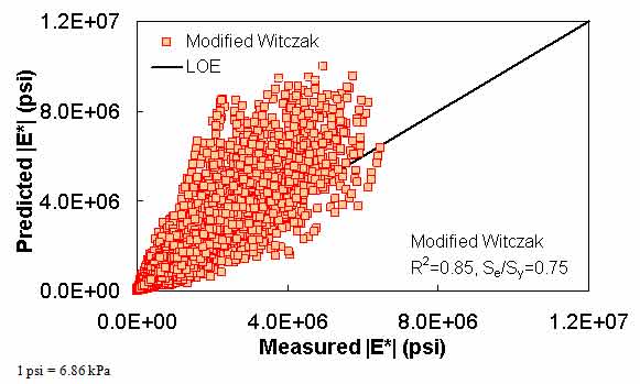
Figure 7. Graph. Prediction of the processed Witczak, FHWA I, FHWA II, NCDOT I, NCDOT II, WRI, and Citgo databases using the modified Witczak in arithmetic scale.
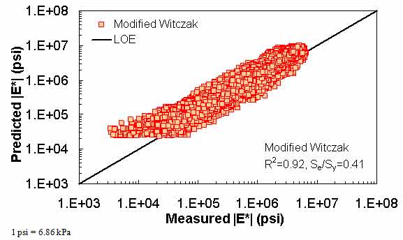
Figure 8. Graph. Prediction of the processed Witczak, FHWA I, FHWA II, NCDOT I, NCDOT II, WRI, and Citgo databases using the modified Witczak in logarithmic scale.
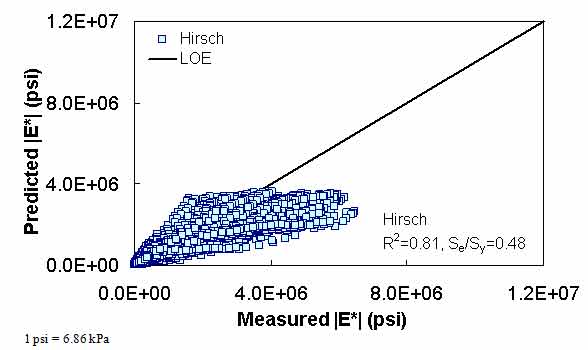
Figure 9. Graph. Prediction of the processed Witczak, FHWA I, FHWA II, NCDOT I, NCDOT II, WRI, and Citgo databases using the Hirsch model in arithmetic scale.
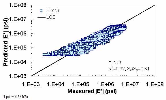
Figure 10. Graph. Prediction of the processed Witczak, FHWA I, FHWA II, NCDOT I, NCDOT II, WRI, and Citgo databases using the Hirsch model in logarithmic scale.
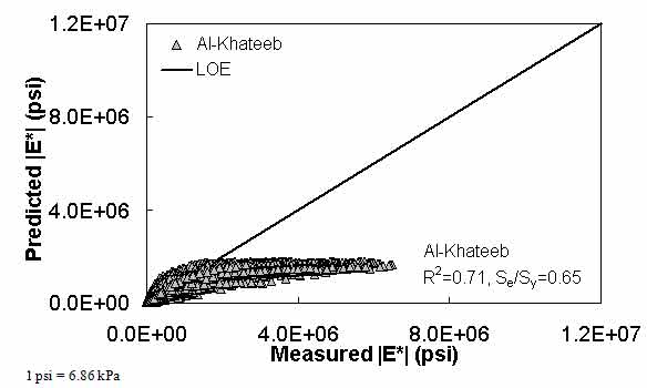
Figure 11. Graph. Prediction of the processed Witczak, FHWA I, FHWA II, NCDOT I, NCDOT II, WRI, and Citgo databases using the Al-Khateeb model in arithmetic scale.
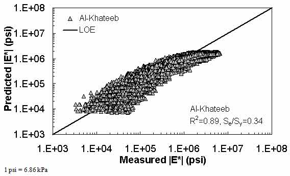
Figure 12. Graph. Prediction of the processed Witczak, FHWA I, FHWA II, NCDOT I, NCDOT II, WRI, and Citgo databases using the Al-Khateeb model in logarithmic scale.
Figure 13. Graph. Prediction of training data containing processed Witczak, FHWA I, NCDOT I, and WRI databases using |G*| binder and gradation-based pilot ANN model (G-GR pANN) in arithmetic scale.
Figure 14. Graph. Prediction of training data containing processed Witczak, FHWA I, NCDOT I, and WRI databases using G-GR pANN in logarithmic scale.
Figure 15. Graph. Prediction of training data containing processed Witczak, FHWA I, NCDOT I, and WRI databases using preliminary |G*|-based models used in phase I of the study (G-V) pANN in arithmetic scale.
Figure 16. Graph. Prediction of training data containing processed Witczak, FHWA I, NCDOT I, and WRI databases using G-V pANN in logarithmic scale.
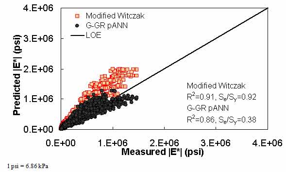
Figure 17. Graph. Predicted moduli using G-GR pANN and modified Witczak models for the FHWA II database in arithmetic scale.
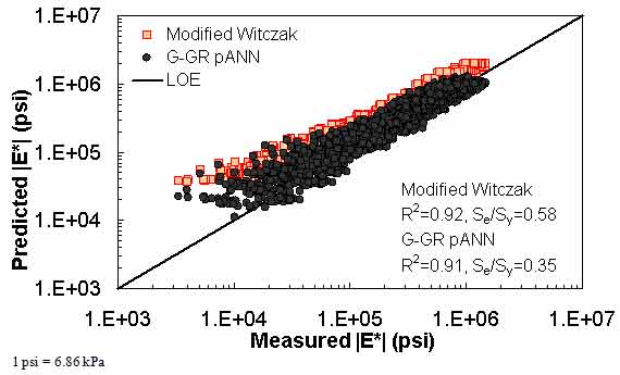
Figure 18. Graph. Predicted moduli using G-GR pANN and modified Witczak models for the FHWA II database in logarithmic scale.
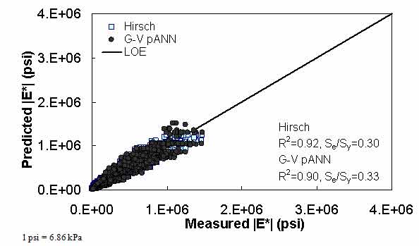
Figure 19. Graph. Predicted moduli using G-V pANN and Hirsch models for the FHWA II database in arithmetic scale.
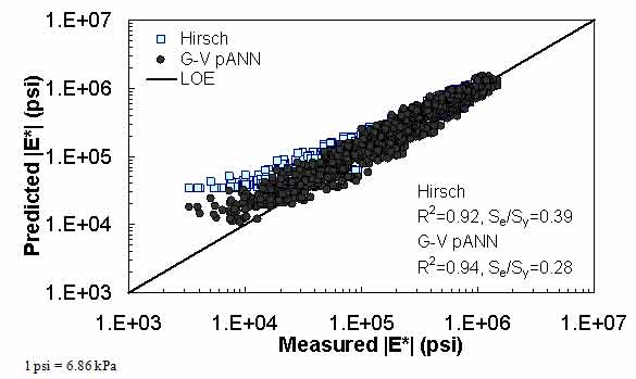
Figure 20. Graph. Predicted moduli using G-V pANN and Hirsch models for the FHWA II database in logarithmic scale.
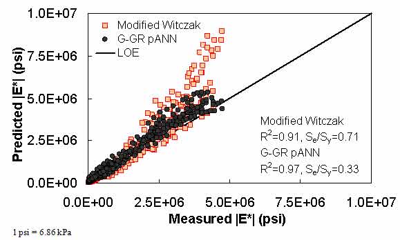
Figure 21. Graph. Predicted moduli using G-GR pANN and modified Witczak models for the NCDOT II database in arithmetic scale.
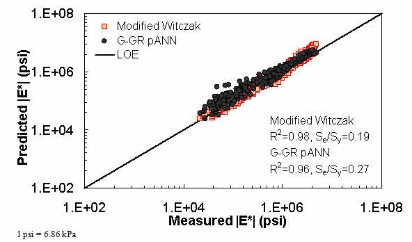
Figure 22. Graph. Predicted moduli using G-GR pANN and modified Witczak models for the NCDOT II database in logarithmic scale.
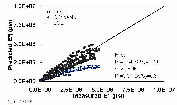
Figure 23. Graph. Predicted moduli using G-V pANN and Hirsch models for the NCDOT II database in arithmetic scale.
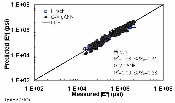
Figure 24. Graph. Predicted moduli using G-V pANN and Hirsch models for the NCDOT II database in logarithmic scale.
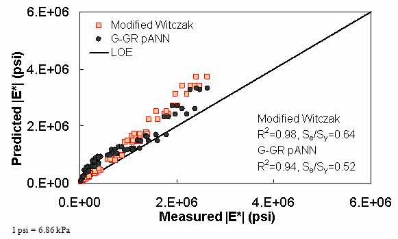
Figure 25. Graph. Predicted moduli using G-GR pANN and modified Witczak models for the Citgo database in arithmetic scale.
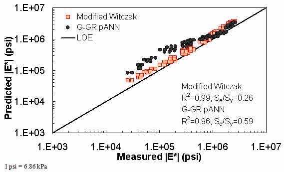
Figure 26. Graph. Predicted moduli using G-GR pANN and modified Witczak models for the Citgo database in logarithmic scale.
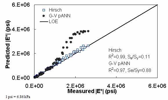
Figure 27. Graph. Predicted moduli using G-V pANN and Hirsch models for the Citgo database in arithmetic scale.
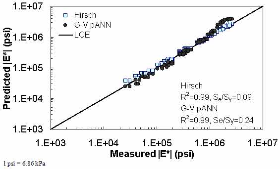
Figure 28. Graph. Predicted moduli using G-V pANN and Hirsch models for the Citgo database in logarithmic scale.
The feasibility of calibrating an ANN using the Hirsch parameters and the modified Witczak model parameters has been investigated. Table 19 shows that the key difference in input requirements for these two models is the lack of gradation parameters for the Hirsch model. Note the naming convention for the ANN models followed in this portion of the report. The first letter group represents the major binder property used (“G” for |G*| and “Visc” for viscosity). The second letter group signifies whether gradation parameters were used (“GR” when they are included and “V” when only volumetric properties are used). Finally, the designation pANN denotes that the model is an ANN model but that it is used only for the pilot studies. The finalized ANN models developed in this project have no prefix before ANN. Due to the issues discussed in appendix C regarding AMPT and TP-62 measured moduli, both types of data were used in the calibration of the ANN model. The calibration results for this model are shown in figure 13 to figure 16, and the verification data are shown in figure 17 to figure 28.
| ANN Model | Parameters Used to Train | Training Database | Verification Database |
|---|---|---|---|
| G-GR pANN | |G*| | FHWA I Processed Witczak1 NCDOT I | FHWA II NCDOT II |
| Va | |||
| Vbeff | |||
| ρ¾ | |||
| ρ3/8 | |||
| ρ4 | |||
| ρ200 | |||
| G-V pANN | |G*| | ||
| VMA (percent) | |||
| VFA (percent) | |||
|
1Portions of the Witczak database (mixtures 1–135) and also some mixtures from the remaining portion that do not have reliable measurements (very high |E*| measurements) were omitted. The portions of the Witczak database used for developing |G*|-based models are the ones that have measured |G*| values. |
|||
For the FHWA II dataset shown in figure 17 and figure 18, the G-GR pANN model shows more scatter than the predictions made from the G-V pANN model and the Hirsch model. Because none of the FHWA II mixtures contain data at 14 °F (-10 °C) (|E*| measurement based on AMPT protocol), there is no observed bias in the Hirsch model shown in figure 19 and figure 20. For the NCDOT II database that contains low temperature data (figure 21 through figure 24), the bias in the Hirsch model is clear. Also, the G-GR pANN and G-V pANN models are similar, with the G-GR pANN model showing a slight improvement both visually and from the statistical measurements.
With the exception of the Citgo dataset, which was discussed previously with regard to the Witczak-based ANNs, the |G*|-based ANN model appears to yield better predictions than the Hirsch and modified Witczak models. The overall performance of this |G*|-based ANN model shows that considering the VMA and VFA parameters together with the t-T dependent binder rheological parameter provides more promising predictions for both the training and verification databases than the parameters used in the modified Witczak model.
The findings from figure 7 to figure 28 are as follows:
Two viscosity-based ANN models with two different sets of parameters were developed (see table 20). The performance of each model is shown in figure 29 through figure 40 for both training and verification databases. Like the |G*|-based ANN models, the difference in these two viscosity-based ANN models are related to the input parameters used for training. In the first ANN, viscosity-gradation (Visc-GR) pANN, the parameters suggested by the original Witczak model are adopted, whereas in the second ANN (viscosity-volumetric (Visc-V) pANN), the Hirsch model parameters are chosen, with the exception that frequency and viscosity are chosen instead of |G*|. Results of the training for the two models are shown in figure 29 to figure 32. Figure 33 to figure 40 show the verification dataset. Note that some of the points used in the training data have also been used in calibrating the original Witczak model. These points represent only a very small portion of the total data shown in figure 29 to figure 32. Results of the independent model verification process are shown for different databases in figure 33 to figure 40. Through these figures, it appears that the ANN models perform better than the original Witczak model. It is also evident that although the Visc-GR pANN model performs better in training, the Visc-V pANN model is better for model verification. Based on these findings, it appears that, like the |G*|-based models, removing gradation parameters from the necessary inputs yielded improved and more stable modulus predictions.
| ANN Model | Parameters Used to Train | Training Database | Verification Database |
|---|---|---|---|
| Visc-GR pANN | f (hertz) | FHWA I Witczak1NCDOT I | FHWA II NCDOT II |
| (109 P) | |||
| Va | |||
| Vbeff | |||
| ρ34 | |||
| ρ38 | |||
| ρ4 | |||
| ρ200 | |||
| Visc-V pANN | f (hertz) | ||
| (109 P) | |||
| VMA (percent) | |||
| VFA (percent) | |||
|
1 Pas = 10 P |
|||
Figure 29. Graph. Prediction of training data containing Witczak, FHWA I, and NCDOT I databases using Visc-GR pANN in arithmetic scale.
Figure 30. Graph. Prediction of training data containing Witczak, FHWA I, and NCDOT I databases using Visc-GR pANN in logarithmic scale.
Figure 31. Graph. Prediction of training data containing Witczak, FHWA I, and NCDOT I databases using Visc-V pANN in arithmetic scale.
Figure 32. Graph. Prediction of training data containing Witczak, FHWA I, and NCDOT I databases using Visc-V pANN in logarithmic scale.
Figure 33. Graph. Predicted moduli using Visc-GR pANN model for the FHWA II database in arithmetic scale.
Figure 34. Graph. Predicted moduli using Visc-GR pANN model for the FHWA II database in logarithmic scale.
Figure 35. Graph. Predicted moduli using Visc-V pANN model for the FHWA II database in arithmetic scale.
Figure 36. Graph. Predicted moduli using Visc-V pANN model for the FHWA II database in logarithmic scale.
Figure 37. Graph. Predicted moduli using Visc-GR pANN model for the NCDOT II database in arithmetic scale.
Figure 38. Graph. Predicted moduli using Visc-GR pANN model for the NCDOT II database in logarithmic scale.
Figure 39. Graph. Predicted moduli using Visc-V pANN model for the NCDOT II database in arithmetic scale.
Figure 40. Graph. Predicted moduli using Visc-V pANN model for the NCDOT II database in logarithmic scale.

