U.S. Department of Transportation
Federal Highway Administration
1200 New Jersey Avenue, SE
Washington, DC 20590
202-366-4000
Federal Highway Administration Research and Technology
Coordinating, Developing, and Delivering Highway Transportation Innovations
| REPORT |
| This report is an archived publication and may contain dated technical, contact, and link information |
|
| Publication Number: FHWA-HRT-11-045 Date: November 2012 |
Publication Number: FHWA-HRT-11-045 Date: November 2012 |
Each ALF test lane can be divided into four quadrants, or sites, as shown in figure 16. FWD testing conducted before placing the asphalt layer and described in subsequent sections indicated variations in unbound layer modulus in sites 1 and 2. General mechanistic-empirical knowledge is that fatigue cracking responses are associated with tensile asphalt strains and can be more influenced by variations in underlying layer properties than can rutting. Therefore, accelerated loading for rutting was conducted in sites 1 and 2, farthest from the parking lot and where the paver began laying the mat. Fatigue loading was conducted in sites 3 and 4, closest to the parking lot, which allowed a longer distance for the paver to place material.
Previous FHWA research illustrated that a wide-base 425 type tire, the kind used in this study, induces greater damage than conventional dual tires.(31) The tires used provide a time-saving advantage in accelerated loading. In addition, the simplicity of a single wheel has advantages in primary response mechanistic-empirical analyses. Different tire inflation pressures and wheel loads were used for rutting and fatigue loading. Fatigue loading utilized a 16,000-lbf (71-kN) wheel load and 120-psi (827-kPa) tire inflation pressure. For rutting, the wheel load and tire inflation pressure were 10,000 lbf (44 kN) and 100 psi (689 kPa), respectively.
The imprint of the tire was measured for the 16,000-lbf (71-kN) wheel load and 120-psi (827‑kPa) tire inflation pressure condition and is shown in figure 22. The effective contact area was between 110.8 and 117.9 inches2 (0.0715 and 0.0761 m2), which was about 80 to 85 percent of the uniformly loaded circular contact area and resulted in an effective contact stress between 150 and 141 psi (1,032 and 971 kPa).
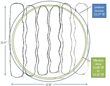
Figure 22. Illustration. Diagram of 425 tire imprint.
Lateral wheel wander of the ALF transverse position is programmable. Three standard deviation tables are available: zero wander, 1.74 inches (50 mm), and 5.25 inches (133 mm). Load applications for rutting did not utilize any wander, and the fatigue loading utilized the 5.25‑inch (133‑mm) standard deviation table. The tables consist of 500 lateral position points randomly normally distributed. The maximum lateral position of the 5.25‑inch (133‑mm) standard deviation table is ±14 inches (356 mm), for a total range of 28 inches (711 mm). When taking into consideration the width of the 425 tire, the transverse extent of the loaded area was 44.6 inches (1,133 mm).
APT experiments must balance practicality with sufficient control on experimental variables. Temperature of the asphalt pavement layers was controlled to the greatest practical extent. Radiant heaters mounted along the length of the ALF were linked to temperature controllers and embedded thermocouples. The target temperatures chosen for rutting and fatigue loading were 147 and 66 °F (64 and 19 °C), respectively. These temperatures were chosen based on the PG temperatures of the variety of asphalt binders.
In the thinner 4-inch (100-mm)-thick pavements, thermocouples were placed at the surface and at depths of 0.78, 1.9, and 3.7 inches (20, 50, and 95 mm). In the thicker 5.8-inch (150-mm)-thick pavements, thermocouples were installed at the surface and at depths of 0.78, 2.9, and 5.6 inches (20, 75, and 145 mm). The thermocouples at the 0.78-inch (20-mm) depth were connected to the closed loop temperature controllers and radiant heaters. Temperature did fluctuate mildly from hourly temperature variations and seasonal variations. Generally, when warming the pavements for 147 °F (64 °C) rutting, the pavement was cooler than the target temperature with depth. The average temperatures at the bottom of the 4- and 5.8-inch (100- and 150-mm) lanes were 144 and 142 °F (62 and 61 °C), respectively. A typical standard deviation at each depth was 2.1 °F (1.2 °C). When the pavement was warmed to keep an intermediate temperature of 66 °F (19 °C) for fatigue cracking, there was a slight warming trend with depth, and the average temperature at the bottom of the 4-inch (100-mm) pavements was 70 °F (21 °C) with a standard deviation of about 2.9 °F (1.6 °C) at various depths.
Rutting was measured at the center of the wheel path without wander. Rut depth was quantified by the change in the thickness of the asphalt layer due to permanent deformation. The layer deformation measurement assembly (LDMA) installed in the asphalt is shown in figure 23. The aluminum plate was installed on top of the CAB before placing the asphalt layers, and holes were drilled through the asphalt layer to the plates after construction. Seven LDMAs were installed per test site.
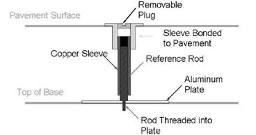
Figure 23. Illustration. LDMA used to measure rut depth.
In addition to the LDMA, rod and level surveys were taken on top of the LDMA to quantify total rutting at the surface. The rut depth of the underlying base and subgrade was then calculated as the difference between the total rod-and-level rut depth and the LDMA asphalt rut depth.
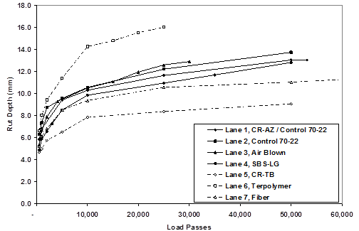
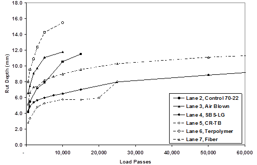
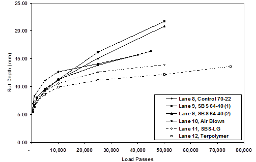
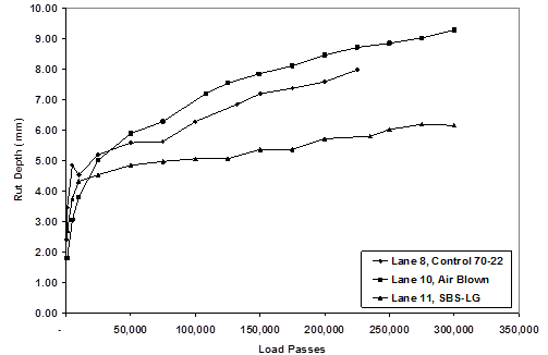
Rut depths from the 147 °F (64 °C) tests on the 4-inch (100-mm)-thick lanes are provided in table 12 and figure 24. Rut depths from the 165 °F (74 °C) tests on the 4-inch (100‑mm)-thick lanes are provided in table 13 and in figure 25. Rut depths from the 147 °F (64 °C) tests on the 5.8-inch (150-mm)-thick lanes are provided in table 14 and in figure 26. Rut depths from the 113 °F (45 °C) tests on 5.8-inch (150-mm)-thick lanes are provided in table 15 and in figure 27.
|
Lane 1, |
Lane 2, |
Lane 3, |
Lane 4, |
Lane 5, |
Lane 6, Terpolymer |
Lane 7, |
|||||||
|---|---|---|---|---|---|---|---|---|---|---|---|---|---|
|
Passes |
Rut Depth (mm) |
Passes |
Rut Depth (mm) |
Passes |
Rut Depth (mm) |
Passes |
Rut Depth (mm) |
Passes |
Rut Depth (mm) |
Passes |
Rut Depth (mm) |
Passes |
Rut Depth (mm) |
|
500 |
5.83 |
500 |
6.27 |
500 |
5.36 |
500 |
4.88 |
500 |
4.66 |
500 |
6.62 |
500 |
5.23 |
|
1,000 |
6.79 |
1,000 |
7.36 |
1,000 |
6.66 |
1,000 |
5.88 |
1,000 |
4.96 |
1,000 |
8.01 |
1,000 |
6.10 |
|
5,000 |
9.41 |
2,000 |
8.71 |
2,000 |
7.88 |
2,000 |
6.53 |
2,000 |
5.75 |
2,000 |
9.41 |
2,000 |
6.79 |
|
10,000 |
10.28 |
5,000 |
9.54 |
4,100 |
9.27 |
3,000 |
7.23 |
5,000 |
6.49 |
5,000 |
11.36 |
5,000 |
8.49 |
|
25,000 |
11.63 |
10,000 |
10.54 |
10,000 |
10.49 |
5,000 |
8.49 |
10,000 |
7.84 |
10,000 |
14.24 |
10,000 |
9.36 |
|
50,000 |
13.02 |
25,000 |
12.19 |
15,000 |
11.06 |
10,000 |
9.84 |
25,000 |
8.36 |
15,000 |
14.76 |
25,000 |
10.54 |
|
53,100 |
13.02 |
50,000 |
13.72 |
20,000 |
11.93 |
25,000 |
10.93 |
50,000 |
9.06 |
20,000 |
15.50 |
50,000 |
11.02 |
|
— |
— |
— |
— |
25,000 |
12.58 |
35,000 |
11.67 |
— |
— |
25,000 |
15.99* |
75,000 |
11.63 |
|
— |
— |
— |
— |
30,000 |
12.89 |
50,000 |
12.80 |
— |
— |
— |
— |
100,000 |
11.84 |
|
— |
— |
— |
— |
— |
— |
— |
— |
— |
— |
— |
— |
125,000 |
12.50 |
1 mm = 0.039 inches
— Indicates test data were not taken because loading had ended.
*Extrapolated.
1 mm = 0.039 inches
Figure 24. Graph. Rut depths for 4-inch (100-mm) lanes at 147 °F (64 °C).
|
Lane 2, |
Lane 3, Air Blown |
Lane 4, |
Lane 5, |
Lane 6, Terpolymer |
Lane 7, |
||||||
|---|---|---|---|---|---|---|---|---|---|---|---|
|
Passes |
Rut Depth (mm) |
Passes |
Rut Depth (mm) |
Passes |
Rut Depth (mm) |
Passes |
Rut Depth (mm) |
Passes |
Rut Depth (mm) |
Passes |
Rut Depth (mm) |
|
500 |
4.18 |
500 |
6.57 |
500 |
4.18 |
500 |
2.79 |
500 |
7.97 |
500 |
5.14 |
|
1,000 |
5.49 |
1,000 |
7.49 |
1,000 |
4.88 |
1,000 |
3.35 |
1,000 |
9.49 |
1,000 |
6.62 |
|
3,000 |
7.18 |
2,000 |
9.06 |
2,000 |
5.40 |
3,000 |
4.79 |
2,000 |
10.89 |
2,000 |
7.32 |
|
5,000 |
7.88 |
3,000 |
9.71 |
3,000 |
5.66 |
5,000 |
5.27 |
3,000 |
12.37 |
3,000 |
7.36 |
|
10,000 |
10.54 |
5,000 |
11.06 |
5,000 |
5.97 |
10,000 |
5.75 |
5,000 |
14.24 |
5,000 |
8.19 |
|
15,000 |
11.50 |
10,000 |
11.76 |
7,500 |
6.27 |
15,000 |
5.70 |
10,000 |
15.46 |
7,500 |
8.67 |
|
— |
— |
— |
— |
10,000 |
6.49 |
20,000 |
5.97 |
— |
— |
10,000 |
8.97 |
|
— |
— |
— |
— |
15,000 |
7.01 |
25,000 |
8.01 |
— |
— |
15,000 |
9.54 |
|
— |
— |
— |
— |
25,000 |
7.97 |
— |
— |
— |
— |
25,000 |
10.28 |
|
— |
— |
— |
— |
50,000 |
8.84 |
— |
— |
— |
— |
50,000 |
11.10 |
|
— |
— |
— |
— |
75,000 |
9.62 |
— |
— |
— |
— |
75,000 |
11.58 |
|
— |
— |
— |
— |
100,000 |
10.49 |
— |
— |
— |
— |
100,000 |
12.10 |
1 mm = 0.039 inches
— Indicates test data were not taken because loading had ended.
1 mm = 0.039 inches
Figure 25. Graph. Rut depths for 4-inch (100-mm) lanes at 165 °F (74 °C).
|
Lane 8, |
Lane 9, Replicate 1, |
Lane 9, Replicate 2, |
Lane 10, |
Lane 11, |
Lane 12, |
||||||
|---|---|---|---|---|---|---|---|---|---|---|---|
|
Passes |
Rut Depth (mm) |
Passes |
Rut Depth (mm) |
Passes |
Rut Depth (mm) |
Passes |
Rut Depth (mm) |
Passes |
Rut Depth (mm) |
Passes |
Rut Depth (mm) |
|
500 |
6.97 |
500 |
5.53 |
1,000 |
6.44 |
500 |
5.62 |
500 |
6.23 |
500 |
6.05 |
|
1,000 |
8.32 |
1,000 |
6.31 |
5,000 |
9.45 |
1,000 |
6.71 |
1,000 |
7.27 |
1,000 |
6.92 |
|
5,000 |
11.10 |
2,000 |
8.06 |
10,000 |
11.15 |
2,000 |
7.32 |
5,000 |
9.19 |
2,000 |
7.36 |
|
10,000 |
12.67 |
5,000 |
9.60 |
25,000 |
15.11 |
5,000 |
9.19 |
10,000 |
10.58 |
5,000 |
8.62 |
|
25,000 |
14.11 |
10,000 |
11.26 |
50,000 |
20.86 |
10,000 |
11.32 |
25,000 |
12.63 |
10,000 |
9.93 |
|
40,000 |
15.68 |
25,000 |
16.22 |
— |
— |
25,000 |
13.85 |
50,000 |
13.93 |
25,000 |
11.15 |
|
— |
— |
50,000 |
21.73 |
— |
— |
45,000 |
16.37 |
— |
— |
50,000 |
12.19 |
|
— |
— |
— |
— |
— |
— |
— |
— |
— |
— |
75,000 |
13.63 |
1 mm = 0.039 inches
— Indicates test data were not measured because loading had ended.
1 mm = 0.039 inches
Figure 26. Graph. Rut depths for 5.8-inch (150-mm) lanes at 147 °F (64 °C).
|
Lane 8, PG70-22 |
Lane 10, Air Blown |
Lane 11, SBS-LG |
|||
|---|---|---|---|---|---|
|
Passes |
Rut Depth (mm) |
Passes |
Rut Depth (mm) |
Passes |
Rut Depth (mm) |
|
500 |
2.39 |
1,000 |
1.79 |
500 |
2.44 |
|
1,000 |
3.44 |
5,000 |
3.05 |
1,000 |
2.70 |
|
5,000 |
4.83 |
10,000 |
3.79 |
5,000 |
3.74 |
|
10,000 |
4.53 |
25,000 |
5.01 |
10,000 |
4.31 |
|
25,000 |
5.18 |
50,000 |
5.88 |
25,000 |
4.53 |
|
50,000 |
5.57 |
75,000 |
6.27 |
50,000 |
4.83 |
|
75,000 |
5.62 |
108,000 |
7.18 |
75,000 |
4.96 |
|
100,000 |
6.27 |
125,000 |
7.53 |
100,000 |
5.05 |
|
132,250 |
6.84 |
149,200 |
7.84 |
125,000 |
5.05 |
|
150,000 |
7.18 |
175,000 |
8.10 |
150,000 |
5.36 |
|
175,000 |
7.36 |
200,000 |
8.45 |
175,000 |
5.36 |
|
200,000 |
7.58 |
225,000 |
8.71 |
200,000 |
5.70 |
|
225,000 |
7.97 |
250,000 |
8.84 |
235,000 |
5.79 |
|
— |
— |
275,000 |
9.01 |
250,000 |
6.01 |
|
— |
— |
300,000 |
9.27 |
275,000 |
6.18 |
|
— |
— |
— |
— |
300,000 |
6.14 |
1 mm = 0.039 inches
— Indicates test data were not measured because loading had ended.
1 mm = 0.039 inches
Figure 27. Graph. Rut depths for 5.8-inch (150-mm) lanes at 113 °F (45 °C).
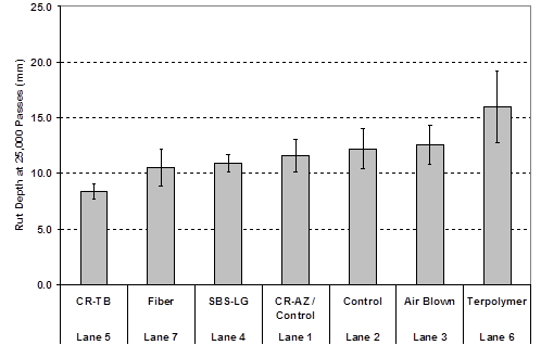
The 147 °F (64 °C) rut tests were the primary rut tests in both thicknesses. The tests began between June and December 2003 and ended between June 2003 and January 2004, except for the first replicate of lane 9 SBS 64-40, which was tested in November 2002. A statistical f‑test and t-test based on the average and standard deviation of rutting between the two replicate tests in lane 9 SBS 64-40 indicated the construction provided statistically equivalent rutting. The rutting performance of all lanes was ranked at 25,000 passes for the primary 147 °F (64 °C) tests with the standard deviation from the seven points of measure, as shown in table 16 and figure 28. Statistical f-tests and t-tests at 95 percent significance were conducted, and the results in table 17 indicate that all lanes provided the same performance statistically except the CR-TB section in lane 5, which was only similar to the fiber section in lane 7. The terpolymer section in lane 6 had similarities with its next two closest ranked sections, air blown in lane 3 and PG70-22 in lane 2.
|
Lane |
Average Rut Depth (mm) |
Standard Deviation Rut Depth (mm) |
|---|---|---|
|
Lane 5, CR-TB |
8.4 |
0.72 |
|
Lane 7, fiber |
10.5 |
1.67 |
|
Lane 4, SBS-LG |
10.9 |
0.78 |
|
Lane 1, CR-AZ/ |
11.6 |
1.47 |
|
Lane 2, PG70-22 |
12.2 |
1.79 |
|
Lane 3, air blown |
12.6 |
1.76 |
|
Lane 6, terpolymer |
16.0 |
3.19 |
1 mm = 0.039 inches
1 mm = 0.039 inches
Figure 28. Graph. Ranked rut depth of 4-inch (100-mm) lanes at 147 °F (64 °C) and 25,000 passes.
|
|
CR-TB |
Fiber |
SBS-LG |
CR-AZ/ PG70-22 |
PG70-22 |
Air Blown |
Terpolymer |
|---|---|---|---|---|---|---|---|
|
CR-TB |
• |
= |
≠ |
≠ |
≠ |
≠ |
≠ |
|
Fiber |
|
• |
= |
= |
= |
= |
≠ |
|
SBS-LG |
|
|
• |
= |
= |
= |
≠ |
|
CR-AZ/ |
|
|
|
• |
= |
= |
≠ |
|
PG70-22 |
|
|
|
|
• |
= |
= |
|
Air Blown |
|
|
|
|
|
• |
= |
|
Terpolymer |
|
|
|
|
|
|
• |
• Trivial self-comparison.
= Statistically equal in rutting at 25,000 passes.
≠ Statistically not equal in rutting at 25,000 passes.
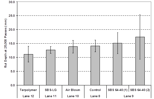
The rutting performance of the 5.8-inch (150-mm) lanes was analyzed with the same methodology. The rutting performance of all lanes was ranked at 25,000 passes for the primary 147 °F (64 °C) tests with the standard deviation from the seven points of measure, as shown in table 18 and figure 29. Statistical f-test and t-test results in table 19 indicate that all lanes provided the same performance except the extreme best and worst performers, terpolymer in lane 12 and the second SBS 64-40 replicate in lane 9. The relative extreme difference in ranked performance of the two 4- and 5.8‑inch (100- and 150-mm) terpolymer sections is an anomaly and is discussed later in this report. Table 20 summarizes the effect of thickness on rutting at 147 °F (64 °C) and compares the average and standard deviation of rutting measured in sections that had the same binder at two thicknesses. Essentially all of the binders rutted the same when placed at 4 and 5.8 inches (100 and 150 mm), except the terpolymer section.
|
Lane |
Average Rut Depth (mm) |
Standard Deviation Rut Depth (mm) |
|
|---|---|---|---|
|
Lane 12, terpolymer |
11.1 |
2.79 |
|
|
Lane 11, SBS-LG |
12.6 |
1.23 |
|
|
Lane 10, air blown |
13.8 |
2.29 |
|
|
Lane 8, PG70-22 |
14.1 |
2.14 |
|
|
Lane 9 |
SBS 64-40 (1) |
15.1 |
3.84 |
|
SBS 64-40 (2) |
17.3 |
8.00 |
|
1 mm = 0.039 inches
1 mm = 0.039 inches
Figure 29. Graph. Ranked rut depth of 5.8-inch (150-mm) lanes at 147 °F (64 °C) and 25,000 passes.
|
|
Terpolymer |
SBS-LG |
Air Blown |
PG70-22 |
SBS 64-40 (1) |
SBS 64-40 (2) |
|---|---|---|---|---|---|---|
|
Terpolymer |
• |
= |
= |
= |
= |
≠ |
|
SBS-LG |
|
• |
= |
= |
= |
= |
|
Air Blown |
|
|
• |
= |
= |
= |
|
PG70-22 |
|
|
|
• |
= |
= |
|
SBS 64-40 (1) |
|
|
|
|
• |
= |
|
SBS 64-40 (2) |
|
|
|
|
|
• |
• Trivial self-comparison.
= Statistically equal in rutting at 25,000 passes.
≠ Statistically not equal in rutting at 25,000 passes.
|
Lane |
100 mm Lanes |
150 mm Lanes |
Statistically Equal |
||
|---|---|---|---|---|---|
|
Rut Depth (mm) |
Standard Deviation (mm) |
Rut Depth (mm) |
Standard Deviation (mm) |
||
|
PG70-22 |
12.2 |
1.8 |
14.1 |
2.1 |
Yes |
|
Air blown |
12.6 |
1.8 |
13.8 |
2.3 |
Yes |
|
SBS-LG |
10.9 |
0.8 |
12.6 |
1.2 |
No |
|
Terpolymer |
16.0 |
3.2 |
11.1 |
2.8 |
No |
1 mm = 0.039 inches
Later in the experiment, rutting tests at 165 and 113 °F (74 and 45 °C) were conducted on select lanes. Although rarely encountered for extended periods of time in the field, the 165 °F (74 °C) rutting temperature provided full-scale rutting performance at the critical or specification temperatures determined by binder rheological tests. The 113 °F (45 °C) rutting temperature provided more realistic conditions for mechanistic-empirical pavement performance prediction analysis. The pavements had undergone some amount of aging between the primary tests at 147 °F (64 °C) and the supplementary tests at 165 and 113 °F (74 and 45 °C). The 165 °F (74 °C) rutting tests on the 4-inch (100-mm) sections began between September and November 2005 and ended between October and November 2005. The terpolymer and air blown sections rutted faster at 165 °F (74 °C) than they did at 147 °F (64 °C). The 113 °F (45 °C) tests on the 5.8-inch (150‑mm) sections began between August and October 2006 and ended between October 2006 and January 2007.
Overall, the effect of changing temperature (and unknown replicate and aging effects) tended to create larger differences between the lanes’ rutting than measured at 147 °F (64 °C). The ranking was essentially the same at 165 and 147 °F (74 and 64 °C), except that the average rutting of fiber in lane 7 and SBS-LG in lane 4 changed rank positions. The control section exhibited slightly less rutting at 165 °F (74 °C) but eventually rutted slightly more than at 147 °F (64 °C). The SBS-LG section had considerably less rutting at 165 °F (74 °C) than at 147 °F (64 °C). The CR-TB section also had less rutting at 165 °F (74 °C) than at 147 °F (64 °C). The fiber section rutting was nearly identical at 165 °F (74 °C) and 147 °F (64 °C). The rutting in the air-blown and terpolymer sections was greater at 165 °F (74 °C) than at 147 °F (64 °C). At 113 °F (45 °C), the rutting was considerably less than at 147 °F (64 °C), and thus, the differences between the sections were considerably less as well. The average ranking between the control, air-blown, and SBS-LG sections was unchanged, with the modified asphalt performing better than the unmodified control and air-blown binder.
Although not utilized in any calculations or quantification in this report, a laser transverse profiler was available to characterize the shape of the rut depth surface. Typical results are shown in figure 30. There was a characteristic upheaval hump on the sides of the wheel path. Exploratory cores were taken from lane 8 and lane 10. Four cores were taken from the center of the wheel path and four cores were taken from the humps. The air void content was calculated using AASHTO T 166 and compared to cores taken from outside the loaded area in the local vicinity of the other cores.(45) The results indicated the rutting increased the density in both the upheaval humps and the wheel path. The air void content of the wheel path decreased about 1.5 percent while the air void content of the humps decreased about 0.5 percent.
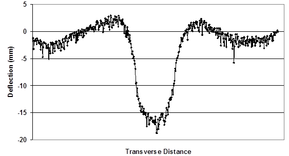
1 mm = 0.039 inches
Figure 30. Graph. Surface profile taken in transverse position across the wheel path of a typical zero wander ALF rut.
Accelerated loading to generate fatigue cracking can take upwards of an order of magnitude more passes than rutting. For perspective, the amount of time to complete 100,000 passes is more than a month, while 10,000 passes takes approximately 5 days. Machine relocations, setup, temperature equilibration, mechanical maintenance, and data collection stops add to the schedule. The ALF devices were stopped at regular intervals for both pavement performance assessment and maintenance. Stops were more frequent earlier in loading to observe immediate changes in rutting or rapid cracking and then were gradually timed farther apart, stopping for machine lubrication.
In January 2003, a shake-down fatigue test was conducted in one of the sites in lane 1 (CR-AZ/ PG70-22). The tire pressure was 110 psi (758 kPa), and the wheel load was 14,000 lbf (62 kN). The section did not exhibit any fatigue cracks after 102,000 passes. Thus, the wheel load and tire pressure were increased. The primary fatigue cracking loading for the thinner, 4-inch (100-mm) sections began between February and December 2004, except for lane 7 (fiber), which began in March 2005. Loading for the thicker, 5.8-inch (150-mm) sections took much longer and had to skip periods during the summer. Two ALFs were used side by side as much as possible. The terpolymer section began in March 2005, but final loading was not complete until July 2006. The air-blown and control sections began in December 2005. Final loading for the air-blown section was completed in May 2006, and final loading for the control section was not complete until March 2008. The SBS-LG and SBS 64-40 sections began loading in January 2007. Final loading for the SBS-LG section was not complete until June 2008, and loading of the SBS 64-40 section ended in July 2007.
Photographs of typical cracked surfaces are shown in figure 31. Cracks were manually traced onto clear Mylar® plastic sheets as they formed at the surface of the pavements. Different color pens were used to correspond to the number of load repetitions. Two approaches were used to process the data. One was to measure the total crack length, and the other was to measure the percentage of area cracked in the loaded area, about 3.4 ft (1 m) wide and 33 ft (10 m) long. A cracked area was considered when individual cracks had grown and met each other, forming a network of cracks. The loaded area was divided into 1- by 1-ft (30- by 30-cm) units to quantify the percent cracked area.
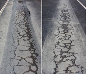
Figure 31. Photo. Typical cracking pattern in loaded ALF wheel paths.
An analysis by Qi et al. found that fatigue cracks begin as small longitudinal cracks.(49) A simplified classification criteria was used to categorize cracks as longitudinal or transverse using a 45‑degree orientation line. Cracks began as longitudinal, and as distributed cracking increased, the orientation became less longitudinal. For example, the ratio of longitudinal to transverse cracks for early loading was as high as 9, but after a significant amount of cracking had occurred toward the end of loading, the ratio was typically around 3. The apparent dominance of longitudinal cracks could be because a single tire was used instead of a dual tire and also because the transverse strain at the bottom of the asphalt layer was tensile while the longitudinal strain transitions from compression to tension and then back to tension as the wheel passes. Repeated tensile-only transverse strains causing longitudinal cracking could be more damaging than any healing from mixed tensile and compressive strains in the other orientation.
Fatigue cracking results at 66 °F (19 °C) for the 4-inch (100-mm) lanes are shown in table 21 and table 22 and graphically in figure 32 and figure 33. Fatigue cracking results at 66 °F (19 °C) for the 5.8-inch (150-mm) lanes are shown in table 23 and table 24 and graphically in figure 34 and figure 35.
|
Lane 1, |
Lane 2, |
Lane 3, |
Lane 4, |
Lane 5, |
Lane 6, Terpolymer |
Lane 7, |
|||||||
|---|---|---|---|---|---|---|---|---|---|---|---|---|---|
|
Passes |
Crack Length (m) |
Passes |
Crack Length (m) |
Passes |
Crack Length (m) |
Passes |
Crack Length (m) |
Passes |
Crack Length (m) |
Passes |
Crack Length (m) |
Passes |
Crack Length (m) |
|
0 |
0.0 |
25,000 |
0.0 |
5,000 |
0.0 |
125,000 |
0.0 |
25,000 |
0.0 |
75,000 |
0.0 |
200,000 |
0.0 |
|
125,000 |
0.0 |
35,000 |
14.3 |
10,000 |
0.8 |
150,000 |
2.0 |
26,000 |
0.1 |
100,000 |
9.2 |
225,000 |
4.0 |
|
150,000 |
0.0 |
50,000 |
31.5 |
25,000 |
13.6 |
175,000 |
9.0 |
35,000 |
1.5 |
125,000 |
13.7 |
250,000 |
8.0 |
|
175,000 |
0.0 |
75,000 |
56.5 |
50,000 |
52.5 |
200,000 |
21.5 |
50,000 |
2.0 |
150,000 |
33.1 |
275,000 |
9.0 |
|
201,000 |
0.0 |
92,100 |
81.4 |
75,000 |
86.5 |
225,000 |
32.0 |
65,000 |
11.3 |
175,000 |
50.0 |
300,000 |
15.2 |
|
225,000 |
0.0 |
100,000 |
90.6 |
93,500 |
108.6 |
250,000 |
39.5 |
75,000 |
13.6 |
200,000 |
66.3 |
— |
— |
|
250,000 |
0.0 |
— |
— |
— |
— |
275,000 |
56.1 |
100,000 |
24.9 |
— |
— |
— |
— |
|
275,000 |
0.0 |
— |
— |
— |
— |
300,000 |
59.8 |
— |
— |
— |
— |
— |
— |
|
375,000 |
0.0 |
— |
— |
— |
— |
— |
— |
— |
— |
— |
— |
— |
— |
1 m = 3.28 ft
— Indicates test data were not measured because loading had ended.
|
Lane 1, |
Lane 2, |
Lane 3, |
Lane 4, |
Lane 5, |
Lane 6, |
Lane 7, Fiber |
|||||||
|---|---|---|---|---|---|---|---|---|---|---|---|---|---|
|
Passes |
Percent Cracked Area |
Passes |
Percent Cracked Area |
Passes |
Percent Cracked Area |
Passes |
Percent Cracked Area |
Passes |
Percent Cracked Area |
Passes |
Percent Cracked Area |
Passes |
Percent Cracked Area |
|
0 |
0.0 |
25,000 |
0.0 |
5,000 |
0.0 |
125,000 |
0.0 |
25,000 |
0.0 |
75,000 |
0.0 |
200,000 |
0.0 |
|
125,000 |
0.0 |
35,000 |
17.7 |
10,000 |
1.0 |
150,000 |
1.1 |
26,000 |
0.0 |
100,000 |
12.5 |
225,000 |
7.3 |
|
150,000 |
0.0 |
50,000 |
38.5 |
25,000 |
15.6 |
175,000 |
7.3 |
35,000 |
1.0 |
125,000 |
14.6 |
250,000 |
9.4 |
|
175,000 |
0.0 |
75,000 |
65.6 |
50,000 |
42.7 |
200,000 |
20.8 |
50,000 |
2.1 |
150,000 |
30.2 |
275,000 |
10.4 |
|
201,000 |
0.0 |
92,100 |
90.6 |
75,000 |
69.8 |
225,000 |
31.3 |
65,000 |
16.7 |
175,000 |
43.8 |
300,000 |
14.6 |
|
225,000 |
0.0 |
100,000 |
100.0 |
93,500 |
78.1 |
250,000 |
37.5 |
75,000 |
18.8 |
200,000 |
59.4 |
— |
— |
|
250,000 |
0.0 |
— |
— |
— |
— |
275,000 |
54.2 |
100,000 |
41.7 |
— |
— |
— |
— |
|
275,000 |
0.0 |
— |
— |
— |
— |
300,000 |
57.3 |
— |
— |
— |
— |
— |
— |
|
375,000 |
0.0 |
— |
— |
— |
— |
— |
— |
— |
— |
— |
— |
— |
— |
—Indicates test data were not measured because loading had ended.
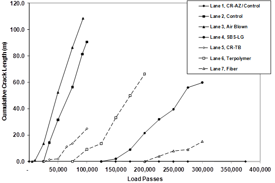
1 m = 3.28 ft
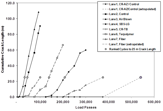
Figure 32. Graph. Cumulative crack length versus ALF passes in 4-inch (100-mm) 66 °F (19 °C) fatigue loaded sections.
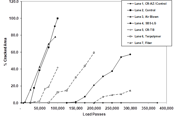
Figure 33. Graph. Percent cracked area versus ALF passes in 4-inch (100-mm) 66 °F (19 °C) fatigue loaded sections.
|
Lane 8, |
Lane 9, |
Lane 10, |
Lane 11, |
Lane 12, Terpolymer |
|||||
|---|---|---|---|---|---|---|---|---|---|
|
Passes |
Crack Length (m) |
Passes |
Crack Length (m) |
Passes |
Crack Length (m) |
Passes |
Crack Length (m) |
Passes |
Crack Length (m) |
|
300,000 |
0.00 |
150,000 |
0.00 |
75,000 |
0.00 |
50,000 |
0.00 |
225,000 |
0.00 |
|
325,000 |
1.00 |
250,000 |
0.00 |
100,000 |
0.25 |
125,000 |
0.00 |
275,000 |
0.00 |
|
425,000 |
3.00 |
340,000 |
0.00 |
125,000 |
7.49 |
200,000 |
0.00 |
400,000 |
0.00 |
|
— |
— |
350,000 |
1.93 |
160,000 |
12.42 |
310,000 |
0.00 |
— |
— |
|
— |
— |
400,000 |
4.88 |
175,000 |
17.75 |
673,000 |
0.00 |
— |
— |
|
— |
— |
425,000 |
6.71 |
200,000 |
25.81 |
— |
— |
— |
— |
|
— |
— |
— |
— |
250,000 |
32.18 |
— |
— |
— |
— |
|
— |
— |
— |
— |
275,000 |
36.02 |
— |
— |
— |
— |
|
— |
— |
— |
— |
300,000 |
41.78 |
— |
— |
— |
— |
|
— |
— |
— |
— |
325,000 |
46.05 |
— |
— |
— |
— |
|
— |
— |
— |
— |
350,000 |
50.37 |
— |
— |
— |
— |
|
— |
— |
— |
— |
375,000 |
52.83 |
— |
— |
— |
— |
1 m = 3.28 ft
— Indicates test data were not measured because loading had ended.
|
Lane 8 |
Lane 9 |
Lane 10 |
Lane 11 |
Lane 12 |
|||||
|---|---|---|---|---|---|---|---|---|---|
|
Passes |
Percent Cracked Area |
Passes |
Percent Cracked Area |
Passes |
Percent Cracked Area |
Passes |
Percent Cracked Area |
Passes |
Percent Cracked Area |
|
300,000 |
0.00 |
150,000 |
0.00 |
100,000 |
0.00 |
50,000 |
0.00 |
225,000 |
0.00 |
|
325,000 |
1.04 |
250,000 |
0.00 |
125,000 |
10.42 |
125,000 |
0.00 |
275,000 |
0.00 |
|
425,000 |
3.13 |
340,000 |
0.00 |
160,000 |
11.46 |
200,000 |
0.00 |
400,000 |
0.00 |
|
— |
— |
350,000 |
1.04 |
175,000 |
15.63 |
673,000 |
0.00 |
— |
— |
|
— |
— |
400,000 |
9.38 |
200,000 |
27.08 |
— |
— |
— |
— |
|
— |
— |
425,000 |
11.46 |
250,000 |
34.38 |
— |
— |
— |
— |
|
— |
— |
— |
— |
275,000 |
35.42 |
— |
— |
— |
— |
|
— |
— |
— |
— |
300,000 |
37.50 |
— |
— |
— |
— |
|
— |
— |
— |
— |
325,000 |
39.58 |
— |
— |
— |
— |
|
— |
— |
— |
— |
350,000 |
45.83 |
— |
— |
— |
— |
|
— |
— |
— |
— |
375,000 |
50.00 |
— |
— |
— |
— |
— Test data were not measured because loading had ended.
1 m = 3.28 ft
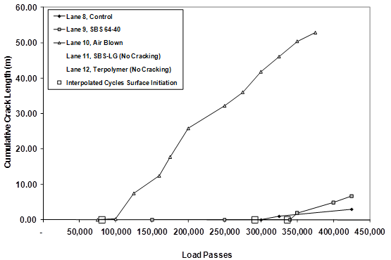
Figure 34. Graph. Cumulative crack length versus ALF passes in 5.8-inch (150-mm) 66 °F (19 °C) fatigue loaded sections.
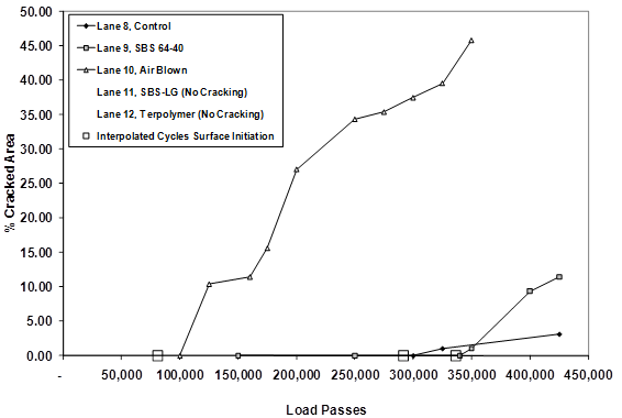
Figure 35. Graph. Percent cracked area versus ALF passes in 5.8-inch (150-mm) 66 °F (19 °C) fatigue loaded sections.
Unlike the rutting performance, there was a more separated variation in the fatigue cracking performance. There is a nearly identical quantitative relationship between the two measures of fatigue cracking; both quantify and rank the performance of the different sections the same. Sections that exhibited surface cracks sooner also developed cracks faster. No cracking was observed for the composite pavement in lane 1 with gap-graded CR-AZ above the dense-graded PG70-22 mixture. Lane 7 (fiber) was very resistant to fatigue cracking and had the least cracking of all the 4-inch (100-mm) sections exhibiting fatigue cracks at the surface. Overall, less cracking and more load passes were required to achieve fatigue crack initiation in the 5.8-inch (150 mm) sections than in the thinner 4-inch (100-mm) sections. Lane 10, with air blown binder, exhibited the largest amount of cracking, as it did in the 4-inch (100-mm) section. The fatigue cracking response of the SBS 64-40 and the PG70-22 binder were intermixed. The lane 8 PG70-22 section had a lower fatigue cracking response curve but achieved surface cracks sooner than lane 9 with SBS 64-40. Cores taken from the PG70-22 section to exhume strain gauges showed delamination at the lift boundary, as shown in figure 36. Lane 11 (SBS-LG) and lane 12 (terpolymer) did not exhibit any surface crack initiation. Cores were also taken from lanes 11 and 12 to look for subsurface bottom-up fatigue cracking that may have initiated but did not propagate through. None of the cores from either lane 11 or 12 indicated that cracking had begun. Some delamination was observed in the cores from lane 11 but less than the cores from lane 8.
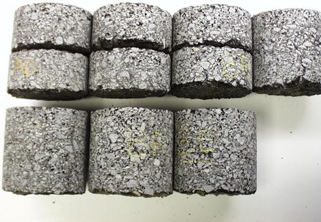
Figure 36. Photo. Cores from lane 8 (PG70-22).
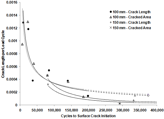
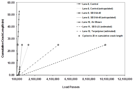
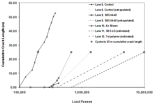
The slope of cracking with passes is plotted against the number of cycles to surface crack initiation in figure 37, which shows two different relationships depending on the thickness of the asphalt. The relationship for the thinner, 4-inch (100-mm) lanes has more points and is better defined than the three points from the thicker, 5.8-inch (150-mm) lanes. In order to build a complete set of rankings for all lanes, extrapolations of this relationship were used to estimate the number of cycles to a 25 percent cracked area and 82 ft (25 m) of cumulative crack length for lanes 1, 11, and 12, which did not exhibit sufficient cracking. The number of cycles to surface crack initiation was taken as the maximum amount of passes applied because the use of any other criteria would be too speculative. Extrapolations from linear regression were used for lanes 7, 8, and 9, for which cracking data were available but not taken to the extent of 25 percent cracked area or 82 ft (25 m) of crack length. The process was fairly straightforward to complete the ranked set for the thinner, 4-inch (100-mm) sections for lane 1. Extrapolations for lanes 11 and 12 were more challenging. Nondestructive seismic evaluation of damage is discussed in chapter 4 and corroborates that lane 11, having received more passes, likely exhibits less damage than lane 12, which received fewer passes. However, when the extrapolated relationship in figure 37 was used along with the maximum passes for lane 11, a comparable number of passes to 25 percent cracked area and 82 ft (25 m) of cracked length were found with lane 9 (SBS 64-40). This is because of the crisscrossed lane 8 and 9 curves and was not accepted because lane 9 exhibited surface cracks, while cores from lane 11 did not show any cracking. Therefore, the slope estimated from figure 37 was taken at only 20 percent of the extrapolated value. Recall that the primary motivation is to obtain a rank order, for which this process was deemed satisfactory. The complete ranking of number of cycles to 25 percent cracked area and 82 ft (25 m) of crack length criteria with the estimations and extrapolations are presented in table 25 and table 26 and shown in figure 38 through figure 43.
1 mm = 0.039 inches
Figure 37. Graph. Crack length developed per load cycle at the point of surface crack initiation.
|
Lane |
Load Passes to Surface Crack Initiation |
Load Passes to 82 ft (25 m) Cumulative Crack |
Load Passes to 25 Percent Cracked Area |
|---|---|---|---|
|
Lane 3, air blown |
6,648 |
32,336 |
33,654 |
|
Lane 2, PG70-22 |
22,728 |
44,311 |
40,250 |
|
Lane 5, CR-TB |
40,178 |
100,297 |
81,818 |
|
Lane 6, terpolymer |
79,915 |
139,583 |
141,667 |
|
Lane 4, SBS-LG |
140,857 |
208,349 |
210,000 |
|
Lane 7, fiber |
185,484 |
375,516 |
379,032 |
|
Lane 1, CR-AZ/PG70-22 |
> 375,000 |
541,405 |
525,075 |
|
Lane |
Load Passes to Surface Crack Initiation |
Load Passes to 82 ft (25 m) Cumulative Crack |
Load Passes to 25 Percent Cracked Area |
|---|---|---|---|
|
Lane 10, air blown |
80,984 |
197,496 |
195,455 |
|
Lane 8, PG70-22 |
291,667 |
1,385,417 |
1,341,667 |
|
Lane 9, SBS 64-40 |
336,326 |
675,602 |
516,091 |
|
Lane 12, terpolymer |
> 400000 |
4,704,085 |
3,285,555 |
|
Lane 11, SBS-LG |
> 673000 |
9,390,351 |
6,682,329 |
1 m = 3.28 ft
Figure 38. Graph. Cumulative crack length of 4-inch (100-mm) lanes with interpolated and extrapolated curves.
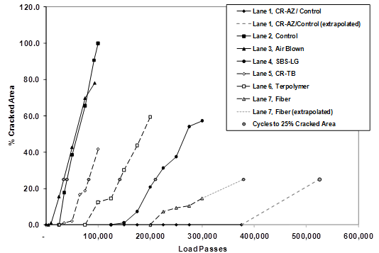
Figure 39. Graph. Percent cracked area of 4-inch (100-mm) lanes with interpolated and extrapolated curves.
1 m = 3.28 ft
Figure 40. Graph. Arithmetic scale plot of cumulative crack length of 5.8-inch (150-mm) lanes with interpolated and extrapolated curves.
1 m = 3.28 ft
Figure 41. Graph. Semilog scale plot of cumulative crack length of 5.8-inch (150-mm) lanes with interpolated and extrapolated curves.
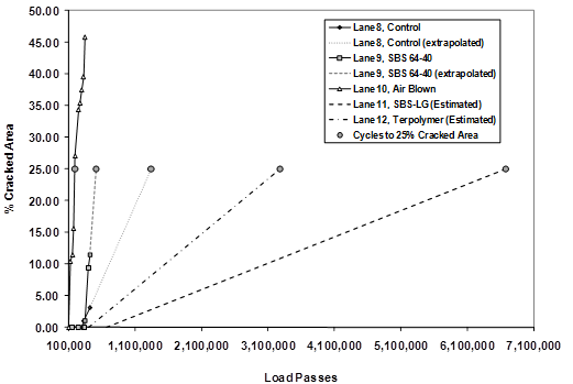
Figure 42. Graph. Arithmetic scale plot of percent cracked area of 5.8-inch (150-mm) lanes with interpolated and extrapolated curves.
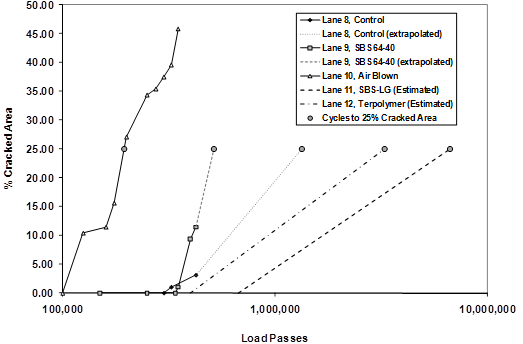
Figure 43. Graph. Semilog scale plot of percent cracked area of 5.8-inch (150-mm) lanes with interpolated and extrapolated curves.
Cores taken from the loaded area of the fatigue loaded sections were examined to confirm that cracks were initiating and then propagating from the bottom of the asphalt layer to the top. Figure 44 shows X-ray computed tomography images of a core taken from a fatigue cracking section. Crack width was larger at the bottom and became thinner toward the surface. Cores from lane 1, with composite pavement of gap-graded CR-AZ above dense graded PG70-22 mix, are shown in figure 45 and indicate that cracks began at the bottom and propagated through the dense-graded PG70-22 mixture, ultimately being arrested or slowed by the CR-AZ layer.
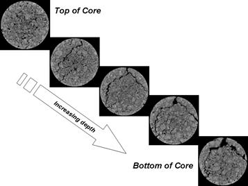
Figure 44. Photo. X-ray computed tomography image slices of an ALF core.
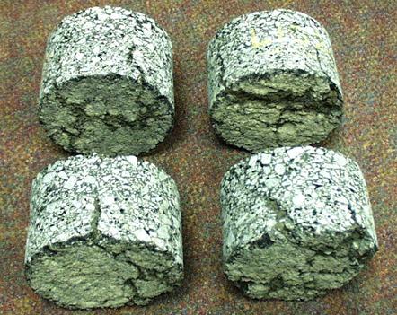
Figure 45. Photo. Cores taken from lane 1.
Rutting occurred and was measured in the fatigue loading sections. The data show smaller rut depth magnitude between 0.16 and 0.32 inches (4 and 8 mm) due to lateral wander and unknown aging effects. Figure 46 and table 27 show the rutting measured in the 4-inch (100-mm)-thick sections during the 66 °F (19 °C) fatigue test. Lane 5 (CR-TB), which performed best during the high-temperature 147 and 165 °F (64 and 74 °C) tests, had the largest and fastest rutting. The other lanes tended to exhibit almost identical behavior up until about 50,000 cycles and then began to diverge. In lane 3 (air blown), rutting increased very rapidly. Lane 4 (SBS-LG) exhibited the best rutting, and lane 6 (terpolymer), which exhibited the worst rutting during the high-temperature tests, was a moderate performer. All of the lanes began the fatigue test during the same year, after about 2 years of aging, but some began early in February while others began in December.
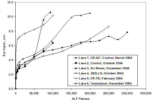
1 mm = 0.039 inches
Figure 46. Graph. Rut depths for 4-inch (100-mm) lanes at 66 °F (19 °C).
|
Lane 1, CR-AZ/ PG70-22 |
Lane 2, |
Lane 3, |
Lane 4, |
Lane 5, |
Lane 6, Terpolymer |
||||||
|---|---|---|---|---|---|---|---|---|---|---|---|
|
Passes |
Rut Depth (mm) |
Passes |
Rut Depth (mm) |
Passes |
Rut Depth (mm) |
Passes |
Rut Depth (mm) |
Passes |
Rut Depth (mm) |
Passes |
Rut Depth (mm) |
|
500 |
1.4 |
1,000 |
1.4 |
500 |
1.7 |
1,000 |
1.6 |
500 |
4.1 |
500 |
1.8 |
|
1,000 |
1.7 |
5,000 |
2.4 |
1,000 |
2.3 |
5,000 |
2.5 |
1,000 |
5.2 |
1,000 |
2.4 |
|
5,000 |
2.7 |
10,000 |
2.8 |
5,000 |
2.6 |
10,000 |
2.9 |
5,000 |
6.9 |
5,000 |
3.3 |
|
10,000 |
3.1 |
25,000 |
3.1 |
10,000 |
3.4 |
25,000 |
3.7 |
10,000 |
7.1 |
10,000 |
3.7 |
|
25,000 |
3.7 |
50,000 |
4.4 |
25,000 |
3.4 |
50,000 |
4.1 |
25,000 |
7.7 |
19,400 |
4.1 |
|
50,000 |
4.4 |
75,000 |
5.2 |
50,000 |
4.5 |
75,000 |
4.5 |
50,000 |
8.2 |
50,000 |
4.7 |
|
75,000 |
5.1 |
100,000 |
6.4 |
75,000 |
9.6 |
100,000 |
4.8 |
75,000 |
8.9 |
75,000 |
5.6 |
|
100,000 |
5.4 |
— |
— |
93,500 |
10.6 |
126,200 |
5.2 |
100,000 |
10.1 |
96,530 |
6.6 |
|
125,000 |
5.7 |
— |
— |
— |
— |
150,000 |
5.8 |
— |
— |
150,000 |
9.9 |
|
150,000 |
6.0 |
— |
— |
— |
— |
175,000 |
6.3 |
— |
— |
175,000 |
10.2 |
|
175,000 |
6.4 |
— |
— |
— |
— |
200,000 |
6.9 |
— |
— |
200,000 |
10.5 |
|
200,000 |
6.5 |
— |
— |
— |
— |
250,000 |
8.6 |
— |
— |
— |
— |
|
225,000 |
6.7 |
— |
— |
— |
— |
— |
— |
— |
— |
— |
— |
|
250,000 |
7.3 |
— |
— |
— |
— |
— |
— |
— |
— |
— |
— |
|
275,000 |
6.8 |
— |
— |
— |
— |
— |
— |
— |
— |
— |
— |
1 mm = 0.039 inches
— Indicates test data were not measured because loading had ended.
Figure 47 and table 28 show the rutting measured in the 5.8-inch (150-mm)-thick sections during the 66 °F (19 °C) fatigue tests. Lane 9 (SBS 64-40), which exhibited the largest amount of rutting during the high-temperature tests at 147 °F (64 °C), provided moderate performance under the intermediate temperatures and wander conditions. It is unknown whether this was due to lane 9 being tested in 2007 rather than with the others in 2005. Lane 11 (SBS-LG) was also tested in 2007, 2 years after the other lanes, and exhibited the best rutting performance. Lane 10 (air blown) clearly performed worst in terms of rutting under the high-temperature zero wander conditions and the intermediate-temperature lateral wander conditions.
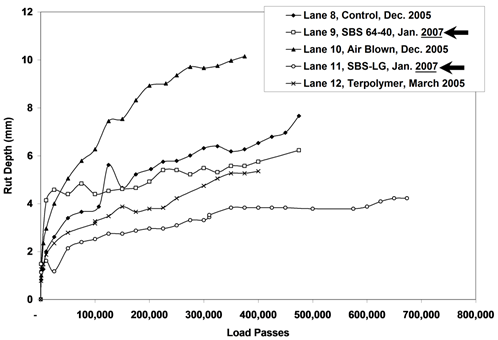
1 mm = 0.039 inches
Figure 47. Graph. Rut depths for 5.8-inch (150-mm) lanes at 66 °F (19 °C).
|
Lane 8, |
Lane 9, |
Lane 10, |
Lane 11, |
Lane 12, Terpolymer |
|||||
|---|---|---|---|---|---|---|---|---|---|
|
Passes |
Rut Depth (mm) |
Passes |
Rut Depth (mm) |
Passes |
Rut Depth (mm) |
Passes |
Rut Depth (mm) |
Passes |
Rut Depth (mm) |
|
1,000 |
0.83 |
1,000 |
1.48 |
1,000 |
1.00 |
1,000 |
1.13 |
500 |
0.78 |
|
5,000 |
1.26 |
10,000 |
4.14 |
5,000 |
2.35 |
10,000 |
1.61 |
1,000 |
1.26 |
|
10,000 |
2.00 |
25,000 |
4.57 |
10,000 |
2.96 |
25,000 |
1.18 |
5,000 |
1.48 |
|
25,000 |
2.61 |
50,000 |
4.40 |
25,000 |
4.01 |
50,000 |
2.13 |
10,000 |
1.87 |
|
50,000 |
3.40 |
75,000 |
4.83 |
50,000 |
5.05 |
75,000 |
2.39 |
25,000 |
2.35 |
|
75,000 |
3.66 |
100,000 |
4.40 |
75,000 |
5.79 |
100,000 |
2.53 |
50,000 |
2.79 |
|
107,000 |
3.88 |
125,000 |
4.53 |
100,000 |
6.27 |
125,000 |
2.74 |
100,000 |
3.18 |
|
125,000 |
5.62 |
150,000 |
4.62 |
125,000 |
7.45 |
150,000 |
2.74 |
100,000 |
3.27 |
|
150,000 |
4.66 |
175,000 |
4.66 |
150,000 |
7.53 |
175,000 |
2.87 |
125,000 |
3.48 |
|
175,000 |
5.23 |
200,000 |
4.92 |
175,000 |
8.32 |
200,000 |
2.96 |
150,000 |
3.88 |
|
203,000 |
5.44 |
225,000 |
5.40 |
200,000 |
8.93 |
225,000 |
2.96 |
175,000 |
3.66 |
|
225,000 |
5.75 |
250,000 |
5.40 |
230,000 |
9.01 |
250,000 |
3.09 |
200,000 |
3.79 |
|
250,000 |
5.79 |
275,000 |
5.23 |
250,000 |
9.36 |
275,000 |
3.31 |
225,000 |
3.83 |
|
275,000 |
6.01 |
300,000 |
5.49 |
275,000 |
9.71 |
300,000 |
3.31 |
250,000 |
4.22 |
|
300,000 |
6.31 |
325,000 |
5.31 |
300,000 |
9.67 |
310,000 |
3.44 |
300,000 |
4.75 |
|
325,000 |
6.40 |
350,000 |
5.57 |
325,000 |
9.75 |
310,000 |
3.53 |
325,000 |
5.05 |
|
350,000 |
6.18 |
375,000 |
5.57 |
350,000 |
9.97 |
350,000 |
3.83 |
350,000 |
5.27 |
|
375,000 |
6.27 |
400,000 |
5.75 |
375,000 |
10.15 |
375,000 |
3.83 |
375,000 |
5.27 |
|
400,000 |
6.53 |
475,000 |
6.23 |
— |
— |
400,000 |
3.83 |
400,000 |
5.36 |
|
425,000 |
6.79 |
— |
— |
— |
— |
425,000 |
3.83 |
— |
— |
|
450,000 |
6.97 |
— |
— |
— |
— |
450,000 |
3.83 |
— |
— |
|
475,000 |
7.66 |
— |
— |
— |
— |
500,000 |
3.79 |
— |
— |
|
— |
— |
— |
— |
— |
— |
575,000 |
3.79 |
— |
— |
|
— |
— |
— |
— |
— |
— |
600,000 |
3.88 |
— |
— |
|
— |
— |
— |
— |
— |
— |
625,000 |
4.09 |
— |
— |
|
— |
— |
— |
— |
— |
— |
650,000 |
4.22 |
— |
— |
|
— |
— |
— |
— |
— |
— |
673,600 |
4.22 |
— |
— |
1 mm = 0.039 inches
— Test data were not measured because loading had ended.
A review of the 147 °F (64 °C) rutting performance of the terpolymer sections in figure 24 and figure 26 shows the rutting in 4-inch (100-mm) lane 6 was significantly larger than other lanes of this thickness. However, the rutting performance of 5.8-inch (150-mm) lane 12 was the smallest and best of that thickness. The rutting performance of 4-inch (100-mm) lane 6 terpolymer appears to be an anomaly and warrants discussion. Earlier research indicated that it is possible to improve laboratory fatigue and permanent deformation performance with this modifier.(50)
The performance of the 5.8-inch (150-mm) lane 12 terpolymer is more in line with expectations, and there does not appear to be enough evidence to suspect anomalous performance in that lane. Youtcheff et al. published an investigation of the performance of 11 modified asphalts in the 2004 Eurasphalt and Eurobitume Conference.(50) The rut resistance was measured using the French pavement rut tester (PRT) and simple shear tester (SST) RSCH, and fatigue was characterized using four-point bending beam fatigue. Moisture damage and permanent deformation were evaluated using Hamburg wheel tracking (HWT). A list of the binders, polymer content, Superpave® PG, and zero shear viscosity (ZSV) are provided in table 29, where terpolymer polymer modifier is also designated by the DuPont™ trade name Elvaloy®. The performance of the mixtures in the French PRT is given in table 29. The terpolymer performed well with smaller rut depth at a given numbers of cycles with some statistical similarities compared to other mixtures. The permanent deformation performance in the SST RSCH is provided in table 30, which shows the terpolymer modified mixture again performed above other binders with some statistical similarities compared to other mixtures. Table 31 lists the fatigue performance in strain-controlled flexural beam fatigue tests, showing the terpolymer modified binder having the best performance at both strain levels. HWT rut depth curves in the paper also show terpolymer having the smallest rut depth at all cycles.(50)
|
Name of Asphalt |
Polymer Content (percent) |
PG |
ZSV 58 °C (Pa·s) |
ZSV 70 °C (Pa·s) |
|---|---|---|---|---|
|
Unmodified PG64 Unmodified PG70-22 |
0 0 |
64-28 70-22 |
903 1,666 |
183 327 |
|
Air-blown asphalt |
0.0 |
70-28 |
3,268 |
530 |
|
Ethylene terpolymer (Elvaloy®) |
2.2 |
76-28 |
6,642 |
1,514 |
|
SBS linear grafted |
3.75 |
70-28 |
2,539 |
490 |
|
SBS linear |
3.75 |
70-28 |
2,088 |
399 |
|
SBS radial grafted |
3.25 |
70-28 |
2,078 |
397 |
|
Ethylene vinyl acetate (EVA) |
5.5 |
64/70-28 |
7,552 |
240 |
|
EVA grafted |
5.5 |
70-28 |
7,267 |
496 |
|
Ethylene styrene interpolymer (ESI) |
5.0 |
76-28 |
2,688 |
625 |
|
Chemically modified crumb rubber asphalt (CMCRA) |
5.0 |
76-28 |
4,304 |
766 |
°F = 1.8(°C) + 32
|
Asphalt Binder or Mixture Designation |
DSR after RTFO Aging |
French PRT after 2 h of STOA |
|||
|---|---|---|---|---|---|
|
High-Temperature PG (°C) |
|G*|/sinδ at 70 °C (Pa) |
Rut Depth at 70 °C (percent) |
|||
|
10.0 radians/s |
0.9 radians/s |
6,000 Passes |
20,000 Passes |
||
|
Elvaloy® |
77 |
4,110 |
753 |
6.5 |
7.9 |
|
Air blown |
74 |
3,870 |
439 |
6.8 |
9.0 |
|
CMCRA |
76 |
4,510 |
566 |
6.8 |
9.7 |
|
EVA |
69 |
1,910 |
203 |
7.1 |
9.4 |
|
SBS radial grafted |
71 |
2,680 |
312 |
7.4 |
8.9 |
|
EVA grafted |
74 |
3,440 |
394 |
7.5 |
10.4 |
|
ESI |
76 |
4,030 |
500 |
7.6 |
9.2 |
|
SBS linear grafted |
72 |
2,880 |
361 |
8.2 |
10.3 |
|
PG70-22 |
71 |
2,640 |
260 |
8.3 |
10.6 |
|
SBS linear |
72 |
2,710 |
309 |
8.5 |
10.5 |
|
PG64-28 |
67 |
1,570 |
151 |
12.1 |
16.0 |
°F = 1.8(°C) + 32
1 Pa = 0.000145 psi
STOA = Short-term oven aging.
|
Asphalt Mixture |
Number of Cycles to Failure Interpolated Actual Fatigue Data |
|G*|sinδ at 19 °C, 10 radians/s (MPa) |
|
|---|---|---|---|
|
At 1,000 microstrains |
At 500 microstrains |
||
|
Elvaloy® |
97,389 |
498,993 |
1.46 |
|
SBS linear grafted |
9,911 |
323,479 |
1.95 |
|
SBS radial grafted |
12,372 |
278,558 |
1.93 |
|
SBS linear |
8,774 |
163,332 |
1.91 |
|
ESI |
10,301 |
135,311 |
0.61 |
|
EVA |
7,147 |
130,817 |
1.01 |
|
Air-blown |
7,614 |
101,436 |
1.61 |
|
CMCRA |
4,158 |
64,751 |
2.55 |
|
EVA grafted |
7,183 |
51,709 |
1.36 |
|
PG64-28 |
5,323 |
37,885 |
2.53 |
|
PG70-22 |
3,144 |
15,877 |
2.31 |
°F = 1.8(°C) + 32
1 MPa = 145 psi
The circumstances of the construction were explored, and a forensic investigation was conducted to avoid any unsubstantiated speculation about the causes of the poor performance. First, both lanes 6 and 12 were constructed on the same date from the same run of plant production. The weather on the day of construction and all relevant preceding days was very good, without any notable rainfall or cold weather. This likely eliminates the possibility that the aggregate stockpiles were saturated when the mix was produced. Chemically speaking, there is no reason to suspect negative interaction of hydrated lime with the terpolymer modifier. The ranking of the rut depths at 165 °F (74 °C) from tests several years after the 147 °F (64 °C) rutting tests was nearly identical; lane 6 had the worst rutting at both points in time. This indicates that the contributing factor to the poor performance is permanent and cannot be linked to any sort of chemical curing of the modifier or to other transient phenomena. Confusingly, the rut performance of 4-inch (100-mm) lane 6 terpolymer at 66 °F (19 °C) was an intermediate performer among the 4-inch (100-mm) sections. This weakly suggests that there could be a high-temperature sensitivity of the mixture in lane 6.
In 2008, cores were taken from lanes 6 and 12. The binder was extracted using trichloroethylene (TCE). The continuous high-temperature PG grade and multiple stress creep and recovery (MSCR) were measured on the extracted binder and compared against RTFO-aged material. Results are summarized in table 32 and indicate that the extracted material is quite different from the original material when inspecting MSCR. The high-temperature PG grades are similar, and the appearance of the discolored aggregate after solvent extraction and marked loss of elasticity suggests that the polymer was not adequately removed from the binder extracted from the field cores. It is important to note that all other unmodified and modified asphalt from this experiment was extracted using TCE without any concerns or discolored aggregate. Nonetheless, both properties of extracted binder from lanes 6 and 12 are fairly comparable, indicating the binder is not substantially different and suggesting that the binder is likely not the cause of the poor performance observed in lane 6.
|
Continuous High-Temperature PG |
RTFO Binder |
Lane 6 Extracted |
Lane 12 Extracted |
||
|---|---|---|---|---|---|
|
74.5 |
74.8 |
71.4 |
|||
|
58 °C |
100 Pa |
JNR, kPa-1 |
— |
0.228 |
0.422 |
|
Percent recovery |
— |
31 |
26 |
||
|
3,200 Pa |
JNR, kPa-1 |
— |
0.247 |
0.47 |
|
|
Percent recovery |
— |
26 |
19 |
||
|
64 °C |
100 Pa |
JNR, kPa-1 |
0.291 |
0.624 |
0.903 |
|
Percent recovery |
69 |
21 |
19 |
||
|
3,200 Pa |
JNR, kPa-1 |
0.362 |
0.736 |
1.074 |
|
|
Percent recovery |
63 |
12 |
8 |
||
|
70 °C |
100 Pa |
JNR, kPa-1 |
0.508 |
1.985 |
2.182 |
|
Percent recovery |
67 |
11 |
11 |
||
|
3,200 Pa |
JNR, kPa-1 |
0.643 |
2.455 |
2.763 |
|
|
Percent recovery |
57 |
0 |
0 |
||
|
76 °C |
100 Pa |
JNR, kPa-1 |
— |
4.654 |
5.181 |
|
Percent recovery |
— |
5 |
4 |
||
|
3,200 Pa |
JNR, kPa-1 |
— |
5.956 |
6.701 |
|
|
Percent recovery |
— |
0 |
0 |
||
°F = 1.8(°C) + 32
1 Pa = 0.000145 psi
— Indicates test were not performed at these temperatures for the RTFO binder.
JNR = Non-recovered compliance.
The average FWD back-calculated modulus of CAB across all lanes was 11,890 psi (82 MPa).
The base modulus calculated in lane 6 for site 1 (147 °F (64 °C) rutting), site 2 (165 °F (74 °C) rutting), site 3 (66 °F (19 °C) fatigue), and site 4 were 8,700; 9,280; 7,395; and 11,600 psi (60, 64, 51, and 80 MPa), respectively. Although site 3 had a low modulus, the modulus in sites 1 and 2 were not dramatically softer than other lanes and sites. For example, the stiffness of the four sites in lane 3 (air blown) were 7,975; 7,830; 7,395; and 8,845 psi (55, 54, 51, and 61 MPa). Again, this lane was unmodified asphalt and did not experience rutting of the magnitude observed in lane 6.
Figure 48 shows a schematic layout of where cores were taken after construction and for a second set of forensic cores. The air void contents of the six cores taken after construction at stations 23, 80, and 139 using saturated surface dry (SSD) AASHTO T 166 of the 4-inch (100-mm) lane 6 were 6.6, 5.5, 7.2, 6.4, 7.0, and 5.8 percent for an average of 6.42 percent and a standard deviation of 0.67 percent.(45) When more cores were taken later from lane 6, the average air void content was 7.6 percent. This was not the largest air void content of the 4-inch (100-mm) sections. The highest average air void content was lane 2, where the average air void content of the six post-construction cores was 7.8 percent with a standard deviation of 0.86 percent. When more cores were taken from lane 2 over time, the average air void content was 8.0 percent. This lane was unmodified asphalt and did not experience rutting of the magnitude observed in lane 6. The average air void content of the 5.8-inch (150-mm) lane 12 terpolymer was 5.9 percent with a standard deviation of 0.91 percent.
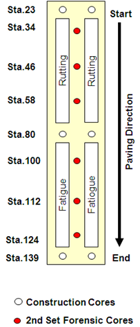
Figure 48. Illustration. Schematic layout of ALF lane construction.
FHWA collaborated with a polymer manufacturer and an asphalt modifying company and supplier, who supplied the terpolymer and modified binder for the experiment, to explore a second set of forensic cores from lane 2 (4 inches (100 mm), PG70-22), lane 6 (4 inches (100 mm), terpolymer), and lane 12 (5.8 inches (150 mm), terpolymer). It was suggested to quantify differences between air void content measured by means of SSD (AASHTO T 166) and CoreLok® (AASHTO T 331).(45,51) Three cores were taken along the centerline of each lane in the rutting sections between sites 1 and 2 at stations 34, 46, and 58. Three cores from each lane were also taken from the fatigue cracking sections between sites 3 and 4 at stations 100, 112, and 124, for a total of 18 cores. The results of FHWA’s tests are shown in table 33.
|
Core Location |
AASHTO T 166(45) (SSD) |
AASHTO T 331(51) (CoreLok®) Air Void (percent) |
Difference in Air Void |
AASHTO T 166(45) Water Absorption (percent) |
|
|---|---|---|---|---|---|
|
Lane 2, |
Station 34 |
9.0 |
9.9 |
0.9 |
2.02 |
|
Station 46 |
6.4 |
7.1 |
0.7 |
0.45 |
|
|
Station 58 |
6.7 |
7.3 |
0.5 |
0.88 |
|
|
Station 100 |
6.4 |
6.9 |
0.5 |
0.72 |
|
|
Station 112 |
6.1 |
6.8 |
0.6 |
0.55 |
|
|
Station 124 |
6.6 |
7.3 |
0.7 |
0.71 |
|
|
Average |
6.9 |
7.5 |
0.7 |
0.9 |
|
|
Lane 6, |
Station 34 |
7.5 |
8.4 |
1.0 |
2.39 |
|
Station 46 |
7.9 |
8.6 |
0.7 |
2.53 |
|
|
Station 58 |
8.1 |
8.8 |
0.7 |
2.99 |
|
|
Station 100 |
8.2 |
8.9 |
0.7 |
2.95 |
|
|
Station 112 |
7.2 |
7.9 |
0.7 |
2.03 |
|
|
Station 124 |
7.6 |
8.1 |
0.5 |
2.02 |
|
|
Average |
7.7 |
8.5 |
0.7 |
2.5 |
|
|
Lane 12, |
Station 34 |
5.2 |
6.2 |
1.0 |
0.98 |
|
Station 46 |
5.4 |
5.8 |
0.4 |
0.95 |
|
|
Station 58 |
5.1 |
5.7 |
0.7 |
0.72 |
|
|
Station 100 |
3.7 |
4.7 |
1.0 |
0.37 |
|
|
Station 112 |
3.5 |
4.2 |
0.6 |
0.26 |
|
|
Station 124 |
4.0 |
4.5 |
0.5 |
0.35 |
|
|
Average |
4.5 |
5.2 |
0.7 |
0.6 |
|
A comparison of the historical SSD air void contents previously described with the second set of forensic cores showed variation but fairly comparable air void contents, with lane 2 having 8 and 6.9 percent, lane 6 having 7.6 and 7.7 percent, and lane 12 having 5.9 and 4.5 percent. As expected, CoreLok® resulted in a larger air void content of 0.7 percent more air voids for all three lanes in the second set of forensic cores. By far, the largest indicator of differences between the anomalous performing lane 6 and better performing lane 12 lay in the water absorption. Lane 6 exhibited over four times larger water absorption than lane 12. Part of that difference may lie in the differences in air void content. However, the air void contents of lanes 2 and 6 were more similar, and the water absorption was still notably higher in lane 6.
Cores from stations 34, 46, and 58 were sent to an asphalt modifying company and supplier for independent testing. Cores from stations 100, 112, and 124 were sent to the FHWA Mobile Asphalt Materials Testing Laboratory (MAMTL) for bulk specific gravity testing using both conventional SSD and CoreLok®. The AASHTO T 166 air void content tests on the whole cores were repeated, and the cores were cut into the top and bottom lifts and measured again.(45) In addition to specific gravity and air void content determination, the individual lifts were tested in a National Center for Asphalt Technology ignition oven to obtain the aggregates so the particle size distribution could be quantified. The air void content, binder content, and water absorption results are shown in table 34, and the extracted aggregate gradations are summarized in table 35 and shown graphically in figure 49.
|
Lane and Station |
Location |
Air Void (percent) |
AASHTO T 166(45) Water Absorption (percent) |
MAMTL Binder Content (percent) |
||||
|---|---|---|---|---|---|---|---|---|
|
TFHRC |
MAMTL |
|||||||
|
AASHTO T 166(45) |
CoreLok® |
AASHTO T 166(45) |
CoreLok® |
TFHRC |
MAMTL |
|||
|
Lane 2-100' CL |
Whole core |
6.4 |
6.9 |
6.9 |
— |
0.72 |
0.79 |
— |
|
Top lift |
— |
— |
7.5 |
8.9 |
— |
1.00 |
5.5 |
|
|
Bottom lift |
— |
— |
5.7 |
5.9 |
— |
0.24 |
5.6 |
|
|
Lane 2-112' CL |
Whole core |
6.1 |
6.8 |
6.7 |
— |
0.55 |
0.74 |
— |
|
Top lift |
— |
— |
7.5 |
8.9 |
— |
1.02 |
5.4 |
|
|
Bottom lift |
— |
— |
5.8 |
6.3 |
— |
0.42 |
5.4 |
|
|
Lane 2-124' CL |
Whole core |
6.6 |
7.3 |
6.9 |
— |
0.71 |
0.73 |
— |
|
Top lift |
— |
— |
7.9 |
9.3 |
— |
1.57 |
5.4 |
|
|
Bottom lift |
— |
— |
5.8 |
5.7 |
— |
0.17 |
5.7 |
|
|
Lane 6-112' CL |
Whole core |
7.2 |
7.9 |
7.6 |
— |
2.03 |
2.51 |
— |
|
Top lift |
— |
— |
8.2 |
9.6 |
— |
3.26 |
5.5 |
|
|
Bottom lift |
— |
— |
6.7 |
6.9 |
— |
1.52 |
5.9 |
|
|
Lane 6-124' CL |
Whole core |
7.6 |
8.1 |
8.1 |
— |
2.02 |
3.05 |
— |
|
Top lift |
— |
— |
8.6 |
9.8 |
— |
3.42 |
5.5 |
|
|
Bottom lift |
— |
— |
6.9 |
6.9 |
— |
1.69 |
5.6 |
|
|
Lane 12-S4-100' |
Whole core |
3.7 |
4.7 |
3.8 |
— |
0.37 |
0.47 |
— |
|
Top lift |
— |
— |
4.8 |
5.3 |
— |
0.98 |
5.5 |
|
|
Bottom lift |
— |
— |
2.0 |
2.6 |
— |
0.07 |
5.8 |
|
|
Lane 12-S4-112' |
Whole core |
3.5 |
4.2 |
3.5 |
— |
0.26 |
0.23 |
— |
|
Top lift |
— |
— |
3.8 |
4.4 |
— |
0.44 |
5.5 |
|
|
Bottom lift |
— |
— |
3.1 |
5.7 |
— |
0.10 |
5.9 |
|
|
Lane 12-S4-124' |
Whole core |
4.0 |
4.5 |
4.2 |
— |
0.35 |
0.34 |
— |
|
Top lift |
— |
— |
4.6 |
5.0 |
— |
0.52 |
5.5 |
|
|
Bottom lift |
— |
— |
3.3 |
3.2 |
— |
0.10 |
5.8 |
|
— Indicates test data were not measured.
CL = Center line of wheel path.
|
Sieve Size |
Lane 2, Total Percent Passing |
Lane 6, Total Percent Passing |
Lane 12, Total Percent Passing |
Limits |
|||||
|---|---|---|---|---|---|---|---|---|---|
|
Std. |
(mm) |
Average |
Std. Dev. |
Average |
Std. Dev. |
Average |
Std. Dev. |
Upper |
Lower |
|
1 inch |
25 |
100.0 |
0.0 |
100.0 |
0.0 |
100.0 |
0.0 |
||
|
3/4 inch |
19 |
100.0 |
0.0 |
100.0 |
0.0 |
100.0 |
0.0 |
||
|
1/2 inch |
12.5 |
95.3 |
0.8 |
96.5 |
0.5 |
96.2 |
0.5 |
||
|
3/8 inch |
9.5 |
85.1 |
1.0 |
89.0 |
0.7 |
88.3 |
1.9 |
||
|
No. 4 |
4.75 |
55.9 |
1.8 |
61.7 |
1.2 |
61.7 |
2.6 |
58 |
52 |
|
No. 8 |
2.36 |
36.0 |
0.9 |
39.5 |
1.2 |
40.6 |
1.9 |
||
|
No. 16 |
1.18 |
25.2 |
0.6 |
27.5 |
0.8 |
28.7 |
1.3 |
||
|
No. 30 |
0.600 |
18.5 |
0.4 |
20.1 |
0.6 |
21.4 |
1.0 |
19 |
15 |
|
No. 50 |
0.300 |
13.7 |
0.3 |
14.8 |
0.5 |
16.0 |
0.8 |
||
|
No. 100 |
0.150 |
9.9 |
0.2 |
10.7 |
0.4 |
11.8 |
0.6 |
||
|
No. 200 |
0.075 |
6.8 |
0.1 |
7.4 |
0.4 |
8.3 |
0.4 |
7 |
5.6 |
1 mm = 0.039 inches
Note: Blank cells indicate there were no gradation limits at the particular sieve size.
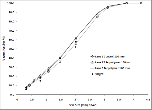
1 mm = 0.039 inches
Figure 49. Graph. Particle size distribution of extracted aggregate for lanes 2, 6, and 12.
The rutting in the asphalt layers was calculated as a percentage of the total surface rutting. The differences in this percentage were evaluated to explore how temperature and wheel wander influence the distribution of permanent deformations in the unbound layers and AC layers. The percentage of total rutting in the asphalt layers for the 4- and 5.8-inch (100- and 150‑mm) lanes at 147 °F (64 °C) and the 4-inch (100-mm) lanes at 165 °F (74 °C) without wander was, on average, 54 percent with a standard deviation of 17 percent. When the temperature was dropped to 113 °F (45 °C) for the 5.8-inch (150-mm) lanes without wander, the percentage of total rutting in the asphalt layer was, on average, 51 percent with a standard deviation of 18 percent. When the temperature was 66 °F (19 °C) with wheel wander, the percentage of rutting in the 4- and 5.8‑inch (100- and 150-mm) asphalt layers was, on average, 31 percent with a standard deviation of 9 percent. The combination of lower temperatures and wheel wander appears to increase rutting in the unbound layers and decrease rutting in the asphalt layers.
This APT experiment was designed with mixtures having identical aggregate and identical mix design with different asphalt binders to allow comparisons to be made between full-scale fatigue cracking and rutting performance and binder specification parameters. The experiment also contains pavement configurations having different thicknesses and stiffnesses (by varying the binder) that allow mechanistic-empirical pavement performance models to be evaluated. Comparisons can be made between measured performance, material property inputs, and design and analysis model outputs that can predict relative and absolute performance.
However, in this experimental design, the initiative of one aspect of the experiment impacts the numerical and statistical strengths of another initiative. A divided subset of pavement test sections by thickness (4 and 5.8 inches (100 and 150 mm)) and the presence of unique types of mixtures and pavements sections (CR-AZ/PG70-22, fiber, CR-TB, and SBS 64-40) that do not have counterparts with a different thickness affect the conditioning of the binder-only variable dataset and the pavement thickness variable dataset. In other words, a statistically sufficient number of data points having only one variable among them are ideal. A total of 12 data points, which correlates to the number of test lanes, is a relatively good number. However, all 12 data points cannot be used for every type of performance comparison, as illustrated in figure 50.
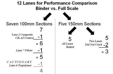
Figure 50. Diagram. Numerical tree of subsets of available comparative data points.
ALF PTF can accommodate 12 lanes, but 7 of the lanes are 4 inches (100 mm) thick, and 5 lanes are 5.8 inches (150 mm) thick. The data from these two sets cannot be easily combined for direct comparison of binder properties against full-scale ALF performance or laboratory mix tests because thickness and constructed density of those lanes confound the binder type variable. The lane 7 fiber mixture cannot be characterized by means of binder tests because the scale of the fibers relative to the size of binder-test specimens is too large for a representative sample. However, the performance of this lane can be utilized for comparisons between laboratory tests on asphalt-aggregate mixtures and full-scale ALF performance. The performance of lane 6 (terpolymer) must be taken with some caution. As shown in the previous section, it had the worst performance of the 4-inch (100-mm) sections but the best performance of 5.8-inch (150-mm) sections, and this poor performance was not within reasonable expectations based on historical binder and mixture tests on the materials. Lane 1 (CR-AZ/PG70-22) is a composite section, which excludes the data from being part of the direct comparison between binder properties and full-scale performance. Naturally, this creates numerical and statistical challenges when it comes to sufficient justification to claim one binder specification parameter is any stronger or weaker than another.
A variety of comparisons and quantitative techniques were used to compare candidate binder specification parameters against mixture performance and full-scale pavement performance. More than one technique summarized in the list below was used because a large number of data points were not available for making comparisons and judging the strength of various material properties against others. Ultimately, the different techniques were combined into a single composite score for simplified cross comparison. The techniques are as follows:
First, the direction of the relationship in either the inverse direction or proportional direction was tested and compared against the direction expected for a particular set of binder parameters and pavement performance quantity. For example, an inverse relationship would be expected for two variables such as amount of cracking in the field versus number of cycles to reach failure in the laboratory. Conversely, a proportional relationship would be expected for two variables such as rut depth at a fixed number of passes versus permanent strain at a fixed number of cycles in the laboratory. The direction of the relationship can be quantified by the linear regression slope, correlation coefficient, and the score calculated by the Kendall’s tau measure of association.
The Kendall’s tau measure of association is a distribution-free, or non-parametric, rank-correlation parameter.(52,53) The parameter is better suited to small datasets than is the correlation coefficient, R, or the coefficient of determination, R2, which are more appropriate for larger datasets. The score is calculated from paired data. The sets of pairs are ranked in increasing order by one of the columns of values. Calculations are based on concordant and discordant observations in the column of data that was not sorted in rank order. All values below the first row are compared to the value in the first row. If the particular value is greater than the first row value, it is considered a concordant observation. Likewise, if the particular value is less than the first row value, it is considered a discordant value. The process is then repeated, but all observations are made relative to the second row value, then to the third row, and so on until the next to last row. The Kendall’s tau score is calculated as shown in figure 51.
![]()
Figure 51. Equation. Kendall’s tau.
Where:
NC = Total number of concordant observations.
ND = Total number of discordant observations.
n = Total number of data points.
The numerical range of Kendall’s tau is between -1 and +1, where a +1 score indicates perfect agreement or ranking between two datasets and a -1 score indicates perfect disagreement or opposite ranking. A score of 0 indicates complete lack of correspondence or complete independence of one dataset from the other. An advantage of the Kendall’s tau parameter is that its magnitude cannot be dominated by isolated data points. The coefficient of determination, R2, can increase (or decrease) rapidly depending on the location of a single data point and artificially suggest a high (or low) degree of correlation even when there are very few data points in a particular set.
Another advantage of the Kendall’s tau parameter is that the statistical significance of the ranking can be evaluated with a statistical test for the independence of the two datasets based on the NC – ND score and the number of paired data points. The null hypothesis, Ho, of the test is that the two datasets are independent of each other and have no correlation. When a single-sided test is used, the alternative hypothesis, Ha, is that the two variables have a correlation greater or less than zero. The basis for the statistics of the Kendall’s tau test for independence comes from the fact that for a given number of data points, there are a fixed number of ranking permutations where there are more possible outcomes with a near-zero score. If Ho is rejected depending on the chosen level of significance in a two-sided test, the correlation of the two sets can be taken as something other than zero. In other words, if more data points were available, some correlation might be expected.
A Kendall’s tau analysis example is given in table 36 and figure 52 with fictitious data. R2 is 0.686, and the slope is -28.686. The magnitude of this value is primarily due to the two data points toward the lower left side increasing the calculated correlation. The Kendall’s tau score is relatively low at -0.2, and the NC – ND score is -3. For n = 6 data points, there are 16 possible NC – ND scores: -15, -13, ‑11, -9, -7, -5, -3, -1, 1, 3, 5, 7, 9, 11, 13, and 15. Similar to a symmetrical normal or Gaussian distribution, there is a greater probability of rank-scores closer to zero and less probability of scores toward the tails, as shown in figure 53, which was reproduced from tables in the literature.(50) The cumulative probability from +1 to +15 is 0.5, and the cumulative probability from -1 to -15 is also 0.5. The single-sided test for either no correlation versus positive (or negative) correlation uses only half of the distribution. As illustrated in figure 54, the cumulative probability or proportion of rankings from -3 to the limit of -15 is 0.36, or 36 percent. It can be concluded that the ranking is only significant at a level of 64 percent (i.e., 100 – 36 percent), whereas statistical significance is customarily judged at 95 percent.
|
Row |
Data X |
Data Y |
Row A |
Row B |
Row C |
Row D |
Row E |
|||||||
|---|---|---|---|---|---|---|---|---|---|---|---|---|---|---|
|
C? |
D? |
C? |
D? |
C? |
D? |
C? |
D? |
C? |
D? |
|||||
|
A |
0.035 |
12.360 |
— |
— |
— |
— |
— |
— |
— |
— |
— |
— |
||
|
B |
0.125 |
18.437 |
✔ |
|
— |
— |
— |
— |
— |
— |
— |
— |
||
|
C |
0.152 |
18.468 |
✔ |
|
✔ |
|
— |
— |
— |
— |
— |
— |
||
|
D |
0.231 |
19.329 |
✔ |
|
✔ |
|
✔ |
|
— |
— |
— |
— |
||
|
E |
0.447 |
5.723 |
|
✔ |
|
✔ |
|
✔ |
|
✔ |
— |
— |
||
|
F |
0.628 |
0.748 |
|
✔ |
|
✔ |
|
✔ |
|
✔ |
|
✔ |
||
|
N |
6 |
|||||||||||||
|
|
6 |
|||||||||||||
|
|
9 |
|||||||||||||
|
NC – ND |
-3 |
|||||||||||||
|
tK |
-0.2 |
|||||||||||||
— Indicates comparison is not used in the mathematics.
C = Concordant; D = Discordant.
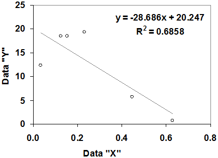
Figure 52. Graph. Fictitious data with linear regression fit for Kendall’s tau rank correlation example.
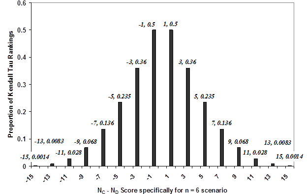
Figure 53. Graph. Possible permutations of rankings for Kendall’s tau.(52)
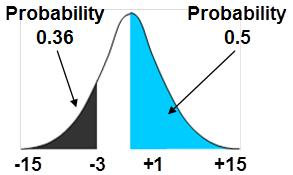
Figure 54. Graph. Continuous area-under-the-curve interpretation for Kendall’s tau.(52)
The ANOVA significance of the regression, or p-value, provides an estimate of the probability that that the slope of the regression curve is not zero or a completely random set of data. The t‑statistic can be calculated from the data using figure 55.
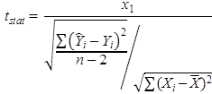
Figure 55. Equation. t-statistic.
Where:
x1 = Fit slope coefficient from regression.
Xi = Individual x-values.
![]() = Average of x-values.
= Average of x-values.
Yi = Individual y-values.
![]() = Predicted y-value.
= Predicted y-value.
n = Number of data points.
The p-value probability is calculated from the statistical t-distribution using two tails and n – 2 degrees of freedom. The significance is 1 minus the probability p-value.
Each of the individual characteristics described is provided for the various comparisons between binder properties against full-scale ALF performance as well as for binder properties against laboratory characterization performance test results. A qualitative composite score can also be calculated considering the variety of statistical measures. While Kendall’s tau score ranges between -1 and +1, the absolute value ranges between 0 and 1. This is also true for the correlation coefficient, R. The statistical significance (probability) of the Kendall’s tau score,
and the statistical significance (probability) of the regression both range between 0 and 1. Therefore, these four parameters can be added together and normalized. Sets of these four scores individually ranging between 0 and 1 can be added together and then divided by the number of scores, yielding a single composite score ranging between 0 and 1 that represents the comparison between the binder candidate parameters against the full-scale ALF performance and the binder candidate parameters against the laboratory performance tests.
A dataset that is familiar and generally accepted by most pavement engineers is the Witczak predictive model for dynamic modulus. This dataset is used to illustrate the variety of statistical measures used to evaluate the candidate binder parameters and mixture characterization tests in light of the full-scale ALF rutting and fatigue performance. The |E*| predictive model has been recently reformulated and recalibrated by Bari.(54) There are 7,400 data points of measured and correspondingly predicted dynamic modulus |E*| shown in log-log scale in figure 56 and in arithmetic scale in figure 57. The slope of the regression is 0.964, which is close to the line of equality, with an intercept of 213,624 psi (1,473 MPa). The R2 value of the fit is 0.90 for the log-log data and 0.80 for the arithmetic data. The ratio of the standard error to the standard deviation of observed values SE/SY is 0.32 for the log-log data and 0.45 for the arithmetic data.
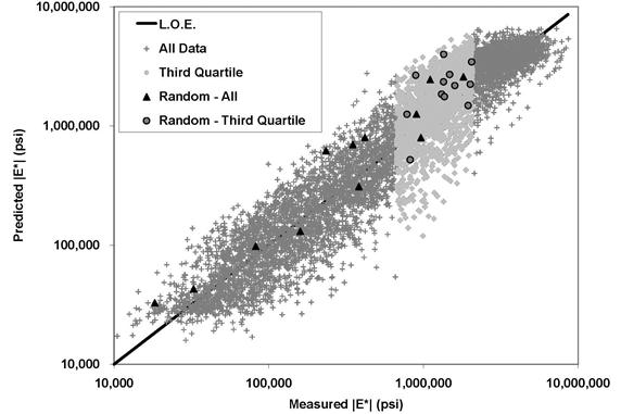
Figure 56. Graph. Log-log plot of measured versus predicted dynamic modulus data points from calibrated Witczak predictive equation.(54)
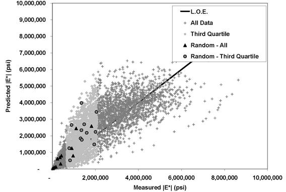
Figure 57. Graph. Arithmetic plot of measured versus predicted dynamic modulus data points from calibrated Witczak predictive equation.(54)
An algorithm was written in MATLAB to conduct four Monte Carlo simulations with 20,000 runs each. Groups of 12 random data points were selected from the entire dataset and again from the third quartile only. This was repeated, but only five random data points were selected from the entire dataset and again from the third quartile. The paired measured and predicted data were ranked in order by measured |E*| and quartiles calculated on the distribution of modulus. The maximum measured dynamic modulus was 8,644,879 psi (59,604 MPa), and the minimum measured dynamic modulus was 10,497 psi (72.4 MPa). The divisions between the first, second, third, and fourth quartiles were 150,297; 666,911; and 2,133,279 psi (1,036; 4,598; and 14,708 MPa). Each quartile had about 1,850 data points. Random points from the entire dataset having a wide range in moduli provided a qualitative analogy to the wide range of good to poor fatigue performance of the various ALF sections. Random points were taken from the third quartile as a qualitative analogy to the rutting performance of the ALF sections where the experimental results produced less diverse rutting performance than fatigue. Sets of 12 data points were used to make a qualitative connection to the 12 ALF lanes. Sets of five data points were used to make a qualitative connection to the small datasets that are comparisons typical of those in this report. In both figure 56 and figure 57, the darker grey points are the entire dataset and the lighter grey points are the third quartile of the data. Graphical examples of 12 random points taken from the data are also shown in the figures.
Kendall’s tau parameter, correlation coefficient, significance of the Kendall’s tau parameter,
and regression p-value were calculated for each of the 20,000 random selections of data points. Then, the frequency of the different values was calculated. The results of the Monte Carlo statistical analyses are shown in table 37 through table 40. The numbers in the first column are the edges of the bins used to sort the Monte Carlo values and calculate the frequency distribution.
|
Kendall’s Tau Coefficient |
12 Points |
5 Points |
||
|---|---|---|---|---|
|
Entire Dataset |
Third Quartile |
Entire Dataset |
Third Quartile |
|
|
-1 |
0.00 |
0.00 |
0.00 |
0.05 |
|
-0.9 |
0.00 |
0.00 |
— |
— |
|
-0.8 |
0.00 |
0.00 |
0.00 |
0.23 |
|
-0.7 |
0.00 |
0.00 |
— |
— |
|
-0.6 |
0.00 |
0.00 |
0.01 |
0.73 |
|
-0.5 |
0.00 |
0.00 |
— |
— |
|
-0.4 |
0.00 |
0.00 |
0.34 |
0.02 |
|
-0.3 |
0.00 |
0.04 |
— |
— |
|
-0.2 |
0.00 |
0.10 |
0.01 |
0.04 |
|
-0.1 |
0.00 |
0.33 |
— |
— |
|
0 |
0.00 |
0.77 |
0.39 |
9.45 |
|
0.1 |
0.00 |
3.11 |
— |
— |
|
0.2 |
0.01 |
5.29 |
1.62 |
16.07 |
|
0.3 |
0.08 |
9.81 |
— |
— |
|
0.4 |
0.32 |
20.59 |
5.89 |
22.94 |
|
0.5 |
1.87 |
20.51 |
— |
— |
|
0.6 |
13.18 |
18.83 |
17.69 |
24.63 |
|
0.7 |
32.21 |
15.58 |
— |
— |
|
0.8 |
39.65 |
4.10 |
39.47 |
18.96 |
|
0.9 |
12.51 |
0.89 |
— |
— |
|
1 |
0.17 |
0.06 |
34.58 |
6.88 |
— Indicates that Kendall’s tau coefficient does not exist when five data points are used.
|
R |
12 Points |
5 Points |
||
|---|---|---|---|---|
|
Entire Dataset |
Third Quartile |
Entire Dataset |
Third Quartile |
|
|
-1 |
0.0 |
0.0 |
0.0 |
0.0 |
|
-0.9 |
0.0 |
0.0 |
0.0 |
0.1 |
|
-0.8 |
0.0 |
0.0 |
0.0 |
0.2 |
|
-0.7 |
0.0 |
0.0 |
0.0 |
0.3 |
|
-0.6 |
0.0 |
0.0 |
0.0 |
0.5 |
|
-0.5 |
0.0 |
0.0 |
0.0 |
0.6 |
|
-0.4 |
0.0 |
0.0 |
0.0 |
0.7 |
|
-0.3 |
0.0 |
0.1 |
0.0 |
1.0 |
|
-0.2 |
0.0 |
0.1 |
0.0 |
1.4 |
|
-0.1 |
0.0 |
0.2 |
0.0 |
1.7 |
|
0 |
0.0 |
0.6 |
0.0 |
2.3 |
|
0.1 |
0.0 |
1.1 |
0.1 |
2.6 |
|
0.2 |
0.0 |
2.2 |
0.2 |
3.3 |
|
0.3 |
0.0 |
3.8 |
0.2 |
4.4 |
|
0.4 |
0.0 |
7.2 |
0.3 |
5.2 |
|
0.5 |
0.0 |
11.2 |
0.7 |
6.7 |
|
0.6 |
0.1 |
16.3 |
1.2 |
8.8 |
|
0.7 |
1.1 |
21.0 |
2.5 |
11.1 |
|
0.8 |
6.0 |
20.9 |
5.9 |
14.3 |
|
0.9 |
28.3 |
13.1 |
15.4 |
16.7 |
|
1 |
64.5 |
2.3 |
73.4 |
18.0 |
|
Kendall’s Tau Significance |
12 Points |
5 Points |
||
|---|---|---|---|---|
|
Entire Dataset |
Third Quartile |
Entire Dataset |
Third Quartile |
|
|
0 |
0.00 |
0.00 |
0.00 |
0.00 |
|
0.1 |
0.00 |
0.00 |
0.00 |
0.00 |
|
0.2 |
0.00 |
0.00 |
0.00 |
0.00 |
|
0.3 |
0.00 |
0.00 |
0.00 |
0.00 |
|
0.4 |
0.00 |
0.40 |
0.00 |
0.00 |
|
0.5 |
0.00 |
2.03 |
0.39 |
8.85 |
|
0.6 |
0.00 |
2.61 |
1.70 |
19.28 |
|
0.7 |
0.00 |
4.03 |
5.90 |
23.18 |
|
0.8 |
0.01 |
13.81 |
17.70 |
23.74 |
|
0.9 |
60.98 |
73.28 |
74.05 |
24.47 |
|
1 |
39.01 |
3.84 |
0.25 |
0.49 |
|
Regression Significance |
12 Points |
5 Points |
||
|---|---|---|---|---|
|
Entire Dataset |
Third Quartile |
Entire Dataset |
Third Quartile |
|
|
0 |
0 |
0 |
0 |
0 |
|
0.1 |
0 |
1 |
0 |
4 |
|
0.2 |
0 |
1 |
0 |
4 |
|
0.3 |
0 |
1 |
0 |
4 |
|
0.4 |
0 |
1 |
0 |
5 |
|
0.5 |
0 |
1 |
0 |
5 |
|
0.6 |
0 |
2 |
1 |
6 |
|
0.7 |
0 |
3 |
1 |
8 |
|
0.8 |
0 |
6 |
2 |
12 |
|
0.9 |
0 |
11 |
7 |
17 |
|
1 |
100 |
74 |
88 |
34 |
Several observations can be made. The distributions of the Kendall’s tau score and correlation coefficient in table 37 and table 38 can be used to interpret the ability of the random sampling to capture the correct (positive) relationship of the true, underlying data. This is essentially the goal of this ALF experiment. The frequencies are summed from -1 to 0 to calculate the likelihood of detecting an incorrect direction of the relationship. Based on the Kendall’s tau score for the following four scenarios: 12 points, all data; 12 points, third quartile; 5 points, all data; and 5 points, third quartile, the likelihoods were 0.00, 1.24, 0.75, and 10.53 percent, respectively. Based on the correlation coefficient, the likelihoods were 0.0, 1.1, 0.2, and 8.8 percent. Naturally, the worst-case scenario happens when few data points are taken from data having a lot of variation relative to the range in values, that is, five data points from the third quartile.
The distributions of the statistical significance calculated from the simulations are given in table 39 for the Kendall’s tau parameter and in table 40 for the regression significance, which is 1 – p-value. It is customary to choose whether to accept or reject at a 95 percent level of significance. Instead, this analysis calculated levels of significance based on the data, which were sometimes larger than 95 percent but most times less than 95 percent. For the same set of data, the Kendall’s tau significance tended to be less than the regression significance. Kendall’s tau significance also tended to be less skewed than the regression significance. This is probably because datasets rarely have very high degrees of rank correlation. However, although there are fewer instances of the highest rank correlation from the Kendall’s tau significance, there appears to be more instances of intermediate to intermediate-high rank correlations. It is clear that the best-case scenario of 12 points taken from the entire dataset guarantees the best likelihood of yielding strong relationships indicative of the true, underlying dataset. In the other extreme, using five data points from a dataset with a lot a variation significantly reduces the likelihood of capturing a meaningful relationship. For this scenario, a mediocre significance level of 70 percent instead of the customary 95 percent may be assumed. In this case, this mediocre level of significance occurs with a likelihood of 71 and 72 percent from both the Kendall’s tau parameter and regression significance calculated when the values from 0.7 to 1 are summed for the scenario of five data points from the third quartile. Although this significance is mediocre, it at least occurs in the majority of the instances.
The intent of this exercise was to provide a qualitative frame of reference for comprehension of the numerical and statistical condition of the datasets in this ALF experiment. Obviously, it is impractical to prepare 30, 300, or 3,000 ALF lanes to identify both the overall population trend and spread in the data that the 12 or 5 lanes are trying to detect. This type of data will never be known. This exercise should also indicate that there are risks to using too few data points but that a less-than-ideal statistical score does not mean there is no underlying relationship at all.