U.S. Department of Transportation
Federal Highway Administration
1200 New Jersey Avenue, SE
Washington, DC 20590
202-366-4000
Federal Highway Administration Research and Technology
Coordinating, Developing, and Delivering Highway Transportation Innovations
| REPORT |
| This report is an archived publication and may contain dated technical, contact, and link information |
|
| Publication Number: FHWA-HRT-11-045 Date: November 2012 |
Publication Number: FHWA-HRT-11-045 Date: November 2012 |
A variety of material characterization tests were conducted on ALF cores, plant-produced mixtures, and laboratory-produced mixtures. This chapter describes both established characterization tests and methodologies that are undergoing development for future applications. Some tests provide a mechanistic engineering property, while others are an empirical qualitative assessment.
The mixture performance is primarily used in chapter 7 to accompany comparisons between binder properties and full-scale ALF performance. These cross-comparisons help capture the degree to which candidate binder parameters (discussed in chapter 5) can discriminate superiority or inferiority in expected performance. In contrast to comparisons between binder properties and full-scale ALF performance, these mixture characterization tests circumvent any influence from less-controlled construction and environmental/climatic variables present at ALF, essentially leveling the playing field by specifically emphasizing the binders’ contribution in a laboratory setting. Characterization of lab-produced mixtures provides more direct comparison to binder variables, especially when the air vocontent of the mixtures is a common fixed value. Characterization of core provides a more direct evaluation of mixture effects on the ALF performance.
The strengths of the various mixture characterization tests are evaluated at the end of this chapter using the statistical techniques described in chapter 3. Composite scores are calculated by comparing the laboratory results against the ALF rutting and cracking performance.
HWT (AASHTO T 324) is a high-temperature, wet submerged test where a steel wheel is reciprocated over surfaces of HMA specimens to evaluate moisture damage and stripping of asphalt binder from the aggregate.(88) This pavement distress is outside the scope of this research. However, the test can also assess the permanent deformation characteristics via the rutting that is induced.
Plant-produced mixtures sampled during construction were compacted in a linear kneading compactor to produce slabs 12 inches (320 mm) long by 10 inches (260 mm) wide and 3 inches (80 mm) thick and having an air void content of 7 percent ±0.5 percent. The water temperature was brought to 147 °F (64 °C), the same temperature as the primary ALF rutting, instead of the cooler temperatures around 104–122 °F (40–50 °C) usually imposed in the test. Typical performance measured in the test is provided in figure 136, where rut depth is measured at individual numbers of cycles. Three replicates were tested, but a fourth was tested for the mixture from lane 6 to achieve a comparison to its corresponding mix in lane 12, and a fourth was tested for lane 8. The ALF mixtures’ performance is quantified by the number of cycles to achieve a 0.4-inch (10-mm) rut depth and is shown in table 74 and figure 137. There are no clear trends in terms of modified and unmodified binders. Performance of the same mixtures placed in different lane thickness is, for the most part, comparable except for the control binder in lanes 2 and 8. Extracted binder contents of those tested specimens were explored between the two lanes and revealed no significant differences to raise concern. Additional HWT tests were conducted on laboratory-prepared materials with 0, 1 (job mix formula), and 1.5 percent hydrated lime to explore the effect of lime distribution and content given the aggregate stockpile dispersion problems described in table 11. The laboratory mixture with 0 percent lime exhibited 5,975 cycles to a 0.4-inch (10-mm) rut, similar to lane 8. The laboratory mixtures with 1.5 and 1.0 percent lime took 15,530 and 12,190 cycles to a 0.4-inch (10-mm) rut, respectively. This suggests that hydrated lime content in lane 8 was less than targeted, which is corroborated by table 11, where the measured lime content was less in lane 8 than in lane 2. The hypothesized net effect is that the lower lime content made the mix vulnerable to poorer than expected performance in this wet stripping test and possibly explains the discrepancy in table 74 and figure 137.
 rut depth plotted on the y-axis and wheel tracking cycles on the x-axis. Three replicate curves from a single mixture are plotted together, and the typical trend is a rapid increase in rut depth that then grows nearly linearly and transitions into a tertiary phase, where rut depth growth accelerates with loading cycles.")
1 mm = 0.039 inches
Figure 136. Graph. HWT rut depth versus wheel tracking cycles.
Binder |
Average Number of Passes to Reach 10-mm Rut Depth at 64 °C |
|||
|---|---|---|---|---|
HMA from 100-mm ALF Sections |
HMA from 150-mm ALF Sections |
|||
Average |
Standard Deviation |
Average |
Standard Deviation |
|
CR-AZ |
9,843 |
816 |
— |
— |
PG70-22 |
20,347 |
6,140 |
5,937 |
367 |
Air blown |
14,900 |
2,025 |
14,092 |
1,983 |
SBS-LG |
8,790 |
1,709 |
9,870 |
1,814 |
CR-TB |
12,593 |
2,525 |
— |
— |
Terpolymer |
9,277 |
2,738 |
6,977 |
934 |
Fiber |
7,017 |
2,373 |
— |
— |
SBS 64-40 |
— |
— |
5,137 |
483 |
°F = 1.8(°C) + 32 1 mm = 0.039 inches
— Indicates test data were not measured.
 test cycles to 4-inch (10-mm) rut depth for plant-produced mixtures. Unfilled bars correspond to mix from 4-inch (100-mm) lanes, and filled bars correspond to mix from 5.8-inch (150-mm) lanes. Error bars represent")
1 mm = 0.039 inches
Figure 137. Graph. HWT test cycles to 4-inch (10-mm) rut depth for plant-produced mixtures.
French PRT is a high-temperature dry wheel tracking test that uses a pneumatic wheel inflated to 87 psi (600 kPa) to reciprocate over slab specimens 20 inches (500 mm) long, 7 inches (180 mm) wide, and 4 or 2 inches (100 or 50 mm) thick. This methodology is used during the French mix design to evaluate mixtures subjected to heavy traffic; mixtures that incorporate materials that tend to lead to rutting, such as some natural sands; and mixtures that have no performance history. It is also used for quality control purposes during construction (see figure 138).
 with a cabinet door opened to show a pneumatic wheel elevated above a rutted test specimen slab.")
Figure 138. Photo. Pneumatic wheel in French PRT and rutted test specimen.
Plant-produced ALF mixtures were compacted to 4-inch (100-mm)-thick slabs at a target air void content of 7 percent ±0.5 percent. The test temperature was 165 °F (74 °C), and the rut depth was manually measured on the surface at 15 locations and averaged. Measurements were taken at 6,000, 20,000, and 60,000 cycles. Two replicate slabs were tested, and the results are summarized in table 75 and figure 139.
Binder |
Rut Depth at 60,000 Passes at 74 °C |
|||
|---|---|---|---|---|
HMA from 100-mm ALF Sections |
HMA from 150-mm ALF Sections |
|||
Average (mm) |
Standard Deviation (mm) |
Average (mm) |
Standard Deviation (mm) |
|
CR-AZ |
8.20 |
0.57 |
— |
— |
CR-AZ composite |
14.30 |
0.99 |
— |
— |
Control (CR-AZ) |
8.20 |
0.14 |
— |
— |
PG70-22 |
8.55 |
1.39 |
11.13 |
1.26 |
Air blown |
8.00 |
0.42 |
8.20 |
1.84 |
SBS-LG |
13.55 |
0.92 |
11.70 |
0.85 |
CR-TB |
6.90 |
0.57 |
— |
— |
Terpolymer |
>20 |
— |
>20 |
— |
Fiber |
15.10 |
1.70 |
— |
— |
SBS 64-40 |
— |
— |
>20 |
— |
°F = 1.8(°C) + 32 1 mm = 0.039 inches
— Indicates test data were not measured.
 for plant-produced mixtures. Unfilled bars correspond to mix from 4-inch (100-mm) lanes, and filled bars correspond to mix from 5.8-inch (150-mm) lanes. Error bars represent one standard deviation.")
1 mm = 0.039 inches
Figure 139. Graph. Rut depth at 60,000 passes in French PRT for plant-produced mixtures.
In general, variability was low. Like HWT, there is no clear trend with respect to modified and unmodified asphalt binders. The soft SBS 64-40 mixture and the terpolymer mixtures from both lanes exceeded the measurable rut depth of 0.8 inches (20 mm) at 60,000 cycles. The thickness of the slabs in this test allowed for composite slabs to reflect the structure of lane 1 CR‑AZ/ PG70-22 in contrast to the thinner slabs in HWT, which do not allow composite slabs to be tested. The slabs with the lane 1 CR-AZ asphalt mixture on top of the PG70-22 mixture provided an average rut depth of 0.558 inches (14.3 mm). When tested by itself, the CR-AZ mixture provided a rut depth of 0.32 inches (8.2 mm). In contrast to the HWT performance, the control mixtures from lanes 2 and 8 were comparable, which strengthens the discussion that lime content differences were captured by the wet HWT. Although the lane 1 control mixture (underneath CR-AZ at ALF) was not tested by the French PRT at a slab thickness of 4 inches (100 mm), the same mixture from lane 2 only had a rut depth of 0.33 inches (8.6 mm). It was speculated that the higher rut depth for the two-layer system was the result of pockets of air voids being trapped between the two layers and of the discontinuity in aggregate structure.
165 °F (74 °C) SST RSCH Lab-Compacted Plant-Produced Mix
RSCH tests were conducted in an SST, and permanent shear strain at 165 °F (74 °C) was measured following AASHTO TP 7-94.(89) A pulsed, haversine shear stress at a level of 10 psi (69.5 kPa) was applied to the test specimens from the horizontal actuator while the vertical actuator applied compression (or tension) to keep the height of the test sample constant. Plant-produced mix sampled from trucks during construction was compacted to 5.26-inch (135-mm)-tall specimens using the Superpave® gyratory compactor. Two specimens 2 inches (50 mm) tall were cut from each gyratory sample, and the target air void content of the final cut samples was 7 percent ±0.5 percent. The loading time was 0.1 s and the rest time was 0.6 s to allow recoverable strains to attenuate and thereby allow the nonrecoverable or permanent shear strain to be measured. The permanent shear strain grows nonlinearly, as shown in figure 140, which illustrates typical data from a less resistant lane 3 (air blown) and a more resistant lane 5 (CR-TB). Five replicates were tested. The tests were carried out until the shear strain limit of the machine was reached or 5,000 cycles.
 repeated shear at constant height (RSCH) test plotted on the y-axis and number of load cycles on the x-axis. Four replicates each from two mixtures are plotted to illustrate typical variation.")
Figure 140. Graph. Permanent shear strain in SST RSCH test versus number of load cycles.
The performance of the ALF mixtures is quantified in table 76 and figure 141 by the number of cycles to reach 20,000 microstrains, equivalent to 2 percent strain. Variability was not consistent and could be either high or low. There is a general trend that the polymer modified binders perform better than the unmodified binders, except the gap-graded CR-AZ mixture. SBS-LG, PG70-22, air-blown, and terpolymer mixtures were placed in both the 4- and 5.8-inch (100- and 150-mm) thickness, and the laboratory performance of these mixtures is comparable, except for the terpolymer mixtures. The SST RSCH laboratory performance of lane 6 terpolymer is better than that of lane 12. This is opposite the French PRT, where the performance was comparable and poor.
Binder |
SST RSCH Cycles to Reach 2 Percent Permanent Shear Strain |
|||
|---|---|---|---|---|
100-mm HMA |
150-mm HMA |
|||
Average |
Standard Deviation |
Average |
Standard Deviation |
|
CR-AZ |
189 |
93 |
— |
— |
PG70-22 |
747 |
239 |
604 |
115 |
Air blown |
537 |
59 |
520 |
39 |
SBS-LG |
1212 |
324 |
1908 |
938 |
CR-TB |
2089 |
734 |
— |
— |
Terpolymer |
3141 |
1857 |
1642 |
365 |
Fiber |
353 |
60 |
— |
— |
SBS 64-40 |
— |
— |
765 |
825 |
1 mm = 0.039 inches
— Indicates tests were not performed.
 repeated shear at constant height (RSCH) cycles to 2 percent (20,000 microstrain) permanent shear strain rut for plant-produced mixtures. Unfilled bars correspond to mix from 4-inch (100-mm) lanes, and filled bars correspond to mix from 5.8-inch (150-mm) lanes. Error bars represent one standard deviation.")
Figure 141. Graph. SST RSCH cycles to 2 percent permanent shear strain rut for plant-produced mixtures.
A full set of field cores from the thicker 5.8-inch (150-mm) ALF sections was taken in 2006, excluding lane 12 because ALF machines were located on top of the lane at the time. The field cores were split into top and bottom lifts and characterized at 147 °F (64 °C) rather than the 165 °F (74 °C) used for plant-produced mixtures. Three replicates were tested, but some lanes and lifts had only two replicates. Plots of the average permanent shear strain curves from the tests for the top and bottom lifts are shown in figure 142 and figure 143, respectively. As expected, there was little variation in the performance of these mixtures, but the general ranking was the same between top and bottom lifts. Table 77 and figure 144 show the average and standard deviation of number of cycles to 2 percent strain (20,000 microstrain) and the microstrain at 200 cycles.
 repeated shear at constant height (RSCH) test plotted on the y-axis and number of load cycles on the x axis. Four curves are plotted, showing the average strain response measured on top lift of 5.8 inch (150-mm)-thick accelerated load facility cores, excluding lane 12.")
Figure 142. Graph. Permanent shear strain in SST RSCH test for top lifts versus number of load cycles.
 repeated shear at constant height (RSCH) test plotted on the y-axis and number of load cycles on the x-axis. Four curves are plotted, showing the average strain response measured on bottom lift of 5.8-inch (150-mm) thick accelerated load facility cores, excluding lane 12.")
Figure 143. Graph. Permanent shear strain in SST RSCH test for bottom lifts versus number of load cycles.
Mix and Lane |
Number of Replicates |
Permanent Shear Strain at 200 Cycles (microstrain) |
Number of Cycles to 20,000 Permanent Shear Microstrain |
|||
|---|---|---|---|---|---|---|
Average |
Standard Deviation |
Average |
Standard Deviation |
|||
Lane 9, SBS 64-40 |
Top |
2 |
16,145 |
106 |
457 |
25 |
Bottom |
3 |
16,243 |
362 |
456 |
49 |
|
Lane 11, SBS-LG |
Top |
3 |
20,160 |
1,552 |
196 |
47 |
Bottom |
3 |
17,003 |
2,407 |
343 |
192 |
|
Lane 10, Air blown |
Top |
3 |
20,110 |
3,152 |
197 |
126 |
Bottom |
3 |
20,243 |
3,357 |
195 |
82 |
|
Lane 8, PG70-22 |
Top |
3 |
20,840 |
4,693 |
180 |
116 |
Bottom |
2 |
23,210 |
3,323 |
138 |
61 |
|

Figure 144. Graph. Permanent shear strain and number of cycles to 20,000 microstrain.
On average, the best performer was the SBS 64-40 lane, followed by the SBS-LG lane. The two unmodified binders, air blown and PG70-22, had the worst performance. However, the differences in the mean performance are reduced by the variability of the test, which is qualitatively the same as the full-scale ALF rutting performance.
Refer to chapter 4 section, "Direct Measurement of Asphalt Layer Modulus," for a discussion of dynamic modulus measured on field cores, plant-produced mixtures, and laboratory-produced mixtures.
The dynamic modulus and phase angle from the plant-produced mixtures, lab-produced mixtures, and field cores are summarized at 66 and 136 °F (19 and 58 °C) both at 0.1 and 10 Hz. The 136 °F (58 °C) data are provided in this section, and the data at 66 °F (19 °C) pertaining to the ALF fatigue cracking tests are in the following section. Only cores from the thicker 5.8-inch (150-mm) lanes could be taken, and the plant-produced fiber mix was no longer available, so only the lab-produced mix is represented. Recall from chapter 4 that the effective frequency of the ALF wheel at various depths and temperatures was between 18 and 3.1 Hz. Although 136 °F (58 °C) was the highest practical temperature for dynamic modulus and is less than the 147 °F (64 °C) ALF rutting test, time-temperature superposition enables the behavior of the materials to be evaluated (see discussion of table 53 in chapter 4).
Cores are always softer than plant-produced and lab-produced mixtures, even though they are more dense (see table 78 and the discussion on compaction effects in chapter 4). The dynamic modulus and phase angle at 136 °F (58 °C) for 10 and 0.1 Hz are shown in table 79 and table 80, respectively. There is no clear trend where plant-produced mixtures are more or less stiff than their lab-produced counterparts.
Dynamic Modulus Specimens |
Air Void Content (percent) |
|
|---|---|---|
Plant-produced samples |
7.0 ±0.5 |
|
Lab-produced samples |
7.0 ±0.5 |
|
Cores |
Lane 8, PG70-22 |
5.1 |
Lane 9, SBS 64-40 |
5.2 |
|
Lane 10, air blown |
3.9 |
|
Lane 11, SBS-LG |
5.3 |
|
Lane 12, terpolymer |
4.5 |
|
Binder |
Specimen Type |
|E*| (MPa) |
Phase Angle (degrees) |
|E*| × sinδ |
|||
|---|---|---|---|---|---|---|---|
Average |
Std. Dev. |
Average |
Std. Dev. |
Average |
Std. Dev. |
||
PG70-22 |
Lab-produced |
360 |
16 |
36.3 |
0.5 |
609 |
33 |
Plant-produced |
303 |
23 |
36.7 |
0.6 |
508 |
46 |
|
Core, lane 8 |
225 |
11 |
36.9 |
1.1 |
375 |
26 |
|
Fiber |
Lab-produced |
351 |
28 |
38.9 |
1.0 |
559 |
35 |
Air blown |
Lab-produced |
437 |
20 |
33.2 |
0.2 |
800 |
39 |
Plant-produced |
420 |
28 |
33.7 |
0.8 |
758 |
57 |
|
Core, lane 10 |
346 |
61 |
34.3 |
0.6 |
615 |
116 |
|
CR-TB |
Lab-produced |
300 |
3 |
31.4 |
0.4 |
577 |
11 |
Plant-produced |
271 |
9 |
32.4 |
0.6 |
505 |
23 |
|
SBS-LG |
Lab-produced |
209 |
33 |
31.9 |
2.5 |
400 |
87 |
Plant-produced |
223 |
— |
31.3 |
— |
430 |
— |
|
Core, lane 11 |
209 |
19 |
33.3 |
0.9 |
381 |
41 |
|
CR-AZ |
Lab-produced |
208 |
19 |
37.8 |
3.1 |
340 |
48 |
Plant-produced |
262 |
49 |
35.1 |
1.6 |
457 |
100 |
|
Terpolymer |
Lab-produced |
168 |
3 |
28.9 |
0.7 |
348 |
2 |
Plant-produced |
197 |
18 |
34.0 |
0.6 |
352 |
33 |
|
Core, lane 12 |
160 |
12 |
34.5 |
0.1 |
282 |
21 |
|
SBS 64-40 |
Lab-produced |
123 |
5 |
27.0 |
1.2 |
270 |
14 |
Plant-produced |
140 |
17 |
31.0 |
1.2 |
273 |
43 |
|
Core, lane 9 |
132 |
21 |
32.5 |
1.6 |
247 |
51 |
|
1 MPa = 145 psi — Indicates only one replicate was available and standard deviation cannot be provided.
Binder |
Specimen Type |
|E*| (MPa) |
Phase Angle (degrees) |
|E*|×sinδ |
|||
|---|---|---|---|---|---|---|---|
Average |
Std. Dev. |
Average |
Std. Dev. |
Average |
Std. Dev. |
||
PG70-22 |
Lab-produced |
59 |
2 |
23.4 |
0.8 |
149 |
10 |
Plant-produced |
52 |
6 |
24.9 |
0.4 |
123 |
15 |
|
Core, lane 8 |
44 |
2 |
21.5 |
1.1 |
121 |
12 |
|
Fiber |
Lab-produced |
46 |
8 |
29.1 |
1.2 |
95 |
18 |
Air blown |
Lab-produced |
80 |
2 |
24.2 |
0.3 |
194 |
3 |
Plant-produced |
67 |
6 |
26.6 |
0.8 |
150 |
18 |
|
Core, lane 10 |
58 |
19 |
26.4 |
2.2 |
134 |
50 |
|
CR-TB |
Lab-produced |
71 |
3 |
23.1 |
0.6 |
181 |
11 |
Plant-produced |
62 |
4 |
23.3 |
1.9 |
159 |
23 |
|
SBS-LG |
Lab-produced |
64 |
13 |
19.7 |
1.9 |
194 |
54 |
Plant-produced |
47 |
— |
21.3 |
— |
130 |
— |
|
Core, lane 11 |
50 |
7 |
22.3 |
1.0 |
132 |
22 |
|
CR-AZ |
Lab-produced |
41 |
6 |
28.1 |
2.2 |
88 |
16 |
Plant-produced |
44 |
6 |
25.9 |
8.1 |
108 |
29 |
|
Terpolymer |
Lab-produced |
65 |
3 |
17.6 |
0.8 |
214 |
17 |
Plant-produced |
54 |
5 |
23.2 |
1.0 |
138 |
14 |
|
Core, lane 12 |
36 |
2 |
25.2 |
1.0 |
84 |
6 |
|
SBS 64-40 |
Lab-produced |
44 |
4 |
18.2 |
0.9 |
142 |
21 |
Plant-produced |
47 |
12 |
23.1 |
6.5 |
130 |
55 |
|
Core, lane 9 |
39 |
10 |
22.4 |
1.9 |
105 |
37 |
|
1 MPa = 145 psi
— Indicates only one replicate was available and standard deviation cannot be provided .
Similar to the binder high-temperature Superpave® PG parameter, |E*|/sinδ was calculated. The modulus-only data at 10 and 0.1 Hz are plotted in figure 145 and figure 146, respectively, which show more variation in stiffness at 10 Hz than at 0.1 Hz. At 10 Hz, the ranking of the |E*| stiffness and |E*|/sinδ are essentially the same whether plant-produced, lab-produced, or field cores, while the error bars representing one standard deviation diminish the differences in mean stiffness. At 0.1 Hz, there is less variation in both |E*| stiffness and |E*|/sinδ, and ranking tends to become less apparent. This is the region of the dynamic modulus master curve that begins to flatten out at high temperatures and low frequencies. Dividing by sinδ at both frequencies tends to normalize the stiffness and diminish the differences between the mixtures, as shown in figure 147 and figure 148.
 and 10 Hz on the y-axis. Three series are plotted, showing data from plant-produced mixtures, lab-produced mixtures, and field cores. Error bars represent one standard deviation.")
1 MPa = 145 psi
Figure 145. Graph. Dynamic modulus |E*| at 136 °F (58 °C) and 10 Hz.
 and 0.1 Hz on the y-axis. Three series are plotted, showing data from plant-produced mixtures, lab-produced mixtures, and field cores. Error bars represent one standard deviation.")
1 MPa = 145 psi
Figure 146. Graph. Dynamic modulus |E*| at 136 °F (58 °C) and 0.1 Hz.
 and 10 Hz on the y-axis. Three series are plotted, showing data from plant-produced mixtures, lab-produced mixtures, and field cores. Error bars represent one standard deviation.")
1 MPa = 145 psi
Figure 147. Graph. |E*|/sinδ at 136 °F (58 °C) and 10 Hz.
 and 0.1 Hz on the y-axis. Three series are plotted, showing data from plant-produced mixtures, lab-produced mixtures, and field cores. Error bars represent one standard deviation.")
1 MPa = 145 psi
Figure 148. Graph. |E*|/sinδ at 136 °F (58 °C) and 0.1 Hz.
Particular attention was paid to evaluating the performance of the ALF mixtures in AMPT (formerly SPT). This includes both dynamic modulus |E*| and flow number tests. AMPT was developed, in part, to overcome the challenges associated with the SST (cost of equipment, required expertise of technicians, pavement design framework, etc.), which was the recommended performance test equipment for the Superpave® system coming out of the SHRP research program. A further benefit of the flow number test is the application of the test results in mechanistic-empirical performance prediction of rutting using methodologies similar to those in the contemporary NCHRP 9-30A, Calibration of Rutting Models for HMA Structural and Mix Design.(90)
Like RSCH, the flow number test is a pulsed cyclic load and recovery test where the permanent strains are measured, but the loading is triaxial compression cycles repeatedly applied to cylindrical test specimens. Idealized behavior in the flow number test is shown in figure 149. Depending on the test conditions, the behavior can exhibit deformation in three regions. The first region is characterized by a large increase in permanent strain, the second region exhibits near linear growth of permanent strain, and the final region is marked by an inflection point and exhibits a more pronounced instability or tertiary flow.
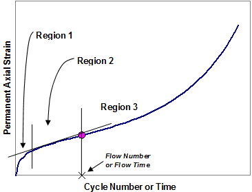
Figure 149. Graph. Permanent axial strain growth in flow number test.
A different strategy from empirical wheel tracking and SST RSCH was taken in the materials and methods for the flow number characterization. As shown in the previous sections, plant-produced mixtures introduced a degree of uncertainty in the laboratory performance due to the lime distribution and production variability. Thus, laboratory-produced specimens were characterized in the flow number test. Also, two groups of specimens were fabricated to allow for both binder comparison and constructed lane comparison where the as-built density was reflected. One group was fabricated to a target air void content of 7 percent ±0.5 percent. The second group was fabricated to the average as-built air void content of each corresponding lane. An overview of the air void content experimental design is provided in table 81. The test temperature for the flow number test was trivially set to 147 °F (64 °C), the same temperature as the primary ALF rutting test in the experiment and, essentially, the upper limit for temperature in AMPT.
Binder Type |
Corresponding Test Lane |
Air Void Content (percent) |
Triaxial Stress |
|
|---|---|---|---|---|
Confining Pressure, |
Deviator Stress, |
|||
| PG70-22 PG70-22 + fiber Air blown CR-TB SBS-LG SBS 64-40 Terpolymer |
General |
7.00 |
69 (10) |
523 (76) |
PG70-22 |
100-mm lane 2 |
8.00 |
69 (10) |
827 (120) |
Air blown |
100-mm lane 3 |
5.75 |
||
SBS-LG |
100-mm lane 4 |
8.00 and 5.50 |
||
CR-TB |
100-mm lane 5 |
7.75 and 5.25 |
||
Terpolymer |
100-mm lane 6 |
7.60 |
||
PG70-22 + fiber |
100-mm lane 7 |
8.00 |
||
PG70-22 |
150-mm lane 8 |
5.00 |
6.9 (1) |
207 (30) |
SBS 64-40 |
150-mm lane 9 |
4.14 |
||
Air blown |
150-mm lane 10 |
5.50 |
||
SBS-LG |
150-mm lane 11 |
5.43 |
||
Terpolymer |
150-mm lane 12 |
5.85 |
||
1 mm = 0.039 inches
Less guidance and application for the flow number test is in practice compared to the established dynamic modulus |E*| stiffness characterization test. As a consequence, the flow number test has been performed with a lack of consensus on stress state and temperature. However, the FHWA Asphalt Mixtures ETG organized a group from industry, agencies, and academia to develop further guidance, an ongoing process at the time this report was written. Depending on the choice of the triaxial stress state and temperature, the flow number test could last a very long time, even without the occurrence of the tertiary flow. Therefore, understanding the mechanism of permanent deformation in asphalt materials and determining the factors that influence the outcomes of the flow number test is an important priority for the research community.
Recently, Gibson et al. developed a more complete understanding of the mechanism of permanent deformation in AC and provided mechanistic-based recommendations for appropriate triaxial stress states for the flow number test.(91) Fully mechanistic, constitutive material models for viscoplasticity (time- and temperature-dependent permanent strains) were used to assess multiaxial stress states that are induced within asphalt layers under truck tires to identify critical locations that yield significantly more deformation than others. Some locations had stress states with larger equivalent deviator stress, which would tend produce larger permanent strains, but equivalent confining stresses in those regions were also larger and tended to reduce the amount of permanent strain from the corresponding deviator stress. Conversely, some locations had smaller equivalent deviator stresses that would produce smaller permanent strains but also had smaller equivalent confining stresses, thereby increasing the amount of permanent strains due to the corresponding deviator stress. The analysis yielded a critical location under the edge of tires a few inches deep, as shown in figure 150.

Figure 150. Illustration. Calculated volumetric permanent strains in a vertical cross sectional plane in the direction of vehicle travel.
A representative equivalent triaxial compression stress state in this region was found to be 10 psi (69 kPa) confinement and 76 psi (523 kPa) axial deviator stress. This stress state was used in the first group of ALF mixtures, with the same 7 percent air void content for all binders, but did not produce a flow number (tertiary flow inflection) within 20,000 cycles. The deviator stress was increased to 120 psi (827 kPa) for the second group of ALF mixtures fabricated to the as-built density of their corresponding lanes in hopes of producing tertiary flow but did not. In addition, the five ALF mixtures prepared for the 5.8-inch (150-mm) HMA sections were tested with a second stress state that was essentially unconfined but with less deviator stress based on estimates from the analysis previously described. Unconfined tests are more convenient given that latex rubber membranes around the specimens are not needed. Gibson et al. includes more discussion on specialty radial strain measurement equipment used in experiments that required a very small (1 psi (7 kPa)) positive confining stress in the essentially unconfined test.(91) Regardless, all tests produced usable permanent deformation curves, even though tertiary flow was only observed in a few mixtures.
Three replicates were tested at each condition. Plots of the average permanent deformation curves for the different mixtures and stress states are provided in figure 151 through figure 153. These data are further reduced in table 82, which quantifies the permanent strain at a fixed number of cycles depending on the test conditions, shown graphically in figure 154 through figure 156.
 confinement, and 76 psi (523 kPa) axial deviator stress. Tertiary flow did not occur.")
Figure 151. Graph. Axial permanent strain versus number of cycles for mixes with 7 percent air void content, 10 psi (69 kPa) confinement, and 76 psi (523 kPa) axial deviator stress.
 confinement, and 120 psi (827 kPa) axial deviator stress. Tertiary flow did not occur.")
Figure 152. Graph. Axial permanent strain versus number of cycles for mixes with as-built air void content, 10 psi (69 kPa) confinement, and 120 psi (827 kPa) axial deviator stress.
 confinement, and 30 psi (207 kPa) axial deviator stress. Tertiary flow occurred in two of the five mixes.")
Figure 153. Graph. Axial permanent strain versus number of cycles for mixes with as-built air void content, 1 psi (6.9 kPa) confinement, and 30 psi (207 kPa) axial deviator stress.
| Binder | Permanent Strain at 20,000 Cycles, 7 Percent Air Void Content | Permanent Strain at 5,000 Cycles Fabricated to As-Built Air Void Content | ||||||
|---|---|---|---|---|---|---|---|---|
| 69 kPa confinement/ 523 kPa axial deviator stress |
69 kPa confinement/827 kPa axial deviator stress | 6.9 kPa confinement/ 207 kPa axial deviator stress |
||||||
| 100-mm ALF Sections | 150-mm ALF Sections | 150-mm ALF Sections (only) | ||||||
| Average | Standard Deviation | Average | Standard Deviation | Average | Standard Deviation | Average | Standard Deviation | |
PG70-22 |
49,303 |
6,450 |
64,340 |
12,196 |
49,615 |
10,355 |
20,138 |
2,470 |
Air blown |
33,741 |
3,782 |
40,260 |
8,804 |
36,576 |
7,249 |
12,391 |
566 |
SBS-LG |
30,421 |
3,890 |
49,773 |
6,761 |
28,814 |
6,639 |
10,274 |
2,070 |
30,429 |
2,228 |
|||||||
CR-TB |
38,420 |
12,662 |
44,071 |
2,736 |
— |
— |
— |
— |
19,965 |
2,001 |
|||||||
Terpolymer |
22,145 |
2,741 |
39,096 |
9,748 |
21,504 |
1,767 |
7,209 |
603 |
Fiber |
34,061 |
1,713 |
45,558 |
3,192 |
— |
— |
— |
— |
SBS 64-40 |
46,210 |
3,477 |
— |
— |
25,076 |
13,960 |
7,365 |
3,610 |
1 kPa = 0.145 psi
1 mm = 0.039 inches
— Indicates tests were not performed.
 mixtures for the condition of fixed 7 percent air voids at 10 psi (69 kPa) confinement and 76 psi (523 kPa) axial deviator stress. Error bars represent one standard deviation.")
Figure 154. Graph. Permanent axial microstrain at 20,000 cycles for ALF mixtures with 7 percent air voids at 10 psi (69 kPa) confinement and 76 psi (523 kPa) axial deviator stress.
 mixtures for the condition of 4-inch (100-mm) ALF as-built air void content at 10 psi (69 kPa) confinement and 120 psi (827 kPa) axial deviator stress. Error bars represent one standard deviation.")
Figure 155. Graph. Permanent axial microstrain at 5,000 cycles for 4-inch (100-mm)
ALF mixtures with as-built air void content at 10 psi (69 kPa) confinement and 120 psi (827 kPa) axial deviator stress.
 accelerated load facility (ALF) mixtures with as-built air void content. Two series of bars are plotted for the two stress state conditions of 10 psi (69 kPa) confinement/120 psi (827 kPa) axial deviator stress and 1 psi (6.9 kPa) confinement/30 psi (207 kPa) axial deviator stress. Error bars represent one standard deviation.")
Figure 156. Graph. Permanent axial microstrain at 5,000 cycles for 5.8-inch (150-mm)
ALF mixtures with as-built air void content.
The permanent deformation performance for the ALF mixtures fabricated to a common 7 percent air void content are ranked in figure 154 from best (terpolymer) to worst (control) along with the standard deviation error bars. Just like the mean ALF rut depth with variability reported in chapter 3, there are quantifiable differences in the average permanent deformation, but the variability reduces the significance of the order of average rut depth.
The mixture-specific flow number characterization tests were used to refine excessively large rut depth predictions by the MEPDG in chapter 4 to explore any benefits that would be provided over the globally calibrated mechanistic-empirical models that rely only on dynamic modulus. The approach taken for the ALF mixtures follows the framework that is being developed in NCHRP 9-30A, although it is not identical given the larger dataset being used for calibration that includes some necessary adjustment factors that are outside the scope of this section.(90)
Power law models were fit to the permanent strain curves measured under the different flow number test conditions. These coefficients allow the lab-measured properties of each mixture to be represented in the MEPDG empirical rutting model shown in figure 157.
![]()
Figure 157. Equation. MEPDG empirical rutting model.
Where:
kz= Depth correction function that adjusts rutting depending on model’s computation.
T = Temperature.
N = Number of passes for a particular vehicle.
k1, k2, k3= Calibration constants.
Elastic recoverable strain, εR, from mechanistic primary response calculations in the MEPDG is used to compute a corresponding plastic irrecoverable strain, εP, by means of the ratio between these two strains in figure 157 rearranged in figure 158.
![]()
Figure 158. Equation. Plastic irrecoverable strain.
First, the strain ratio, which can be found specifically from laboratory tests, is equated to the same ratio that is used in the MEPDG (see figure 159). Figure 160 illustrates how the power law form that represents the laboratory flow number test is substituted for ![]() P in figure 159.
P in figure 159.

Figure 159. Equation. Equivalence assumed between laboratory performance and MEPDG mechanistic-empirical model formulation.

Figure 160. Equation. Equating laboratory test power law permanent deformation parameters with MEPDG mechanistic-empirical model formulation.
Next, it is necessary to produce the equivalent laboratory-based recoverable strain from the lab test in figure 160 using the dynamic modulus master curves of the mixtures and the deviator stresses applied in the flow number tests, as shown in figure 161.
![]()
Figure 161. Equation. Derivation of recoverable strain for MEDPG mechanistic-empirical permanent deformation model based on applied stress in flow number test and dynamic modulus.
The dynamic modulus of HMA is sensitive to confining pressure as well as to other variables. Thus, the unconfined dynamic modulus would not be entirely appropriate to use in figure 161 when the confined flow number tests are being used in this approach. Kim et al. quantified the sensitivity of dynamic modulus to confining pressure, as shown in figure 162, where modulus increases in the high-temperature, low-frequency region of the dynamic modulus master curve.(92) Based on this data, it was assumed that dynamic modulus increases by a factor of 2 at 147 °F (64 °C) and frequency is equivalent to the load pulse in the flow number test.
 confining stress applied during the test. All master curves coalesce at intermediate and high reduced frequency but diverge at lower frequencies, which also represent higher temperatures. In this region, the increase in confining stress is reflected with an increase in dynamic modulus.")
1 MPa = 145 psi
Figure 162. Graph. Dynamic modulus versus reduced frequency.(92)
The depth correction factor kz in figure 160 was ignored in the following derivations, and the elastic recoverable strain term determined from the laboratory flow number tests was incorporated into the modified power law multiplier term a', as shown in figure 163.
![]()
Figure 163. Equation. Equating laboratory test power law permanent deformation parameters with MEPDG mechanistic-empirical model formulation (continued from figure 160).
From figure 163, it can be determined that the exponent on the power law b fit to the flow number data can be used as k3 in the MEPDG. The temperature term was also left alone in this approach because laboratory tests were only conducted at 147 °F (64 °C), and the value k2 = 1.506 in the MEPDG was calibrated with more temperature conditions. Finally, the value for k1 was determined using the modified power law multiplier a', k2, and the temperature of the flow number test in degrees Fahrenheit, as illustrated in figure 164.

Figure 164. Equation. Derivation of k1 term for MEPDG mechanistic-empirical model for rutting based on laboratory test conditions
Table 83 shows all of the power law coefficients fit to flow numbers, modulus, and strain values used to determine the mixture specific k1 and k3 for the MEPDG, shown in table 84.
| Mix | 64 °C Modulus (kPa) | Recoverable Strain (microstrain) | Power Law Coefficients Fit to Flow Number Data | ||||
|---|---|---|---|---|---|---|---|
| 69/827 kPa | 6.9/207 kPa | ||||||
| 6.9 kPa Confinement | 69 kPa Confinement | a | b | a | b | ||
Lane 2 |
180,594 |
1,146 |
2,290 |
1329.9 |
0.446 |
— |
— |
Lane 3 |
253,465 |
817 |
1,631 |
2920.7 |
0.309 |
— |
— |
Lane 4 |
164,323 |
1,260 |
2,516 |
3106.6 |
0.265 |
— |
— |
Lane 5 |
365,015 |
567 |
1,133 |
2730.9 |
0.320 |
— |
— |
Lane 6 |
125,926 |
1,644 |
3,284 |
4181.0 |
0.253 |
— |
— |
Lane 8 |
192,150 |
1,077 |
2,152 |
2228.4 |
0.358 |
803.9968 |
0.385196 |
Lane 9 |
125,802 |
1,645 |
3,287 |
3463.6 |
0.258 |
1638.743 |
0.225394 |
Lane 10 |
293,289 |
706 |
1,410 |
2464.8 |
0.323 |
551.3707 |
0.397649 |
Lane 11 |
181,215 |
1,142 |
2,282 |
3920.9 |
0.226 |
1568.197 |
0.219232 |
Lane 12 |
145,914 |
1,419 |
2,834 |
4565.6 |
0.185 |
2500.387 |
0.144622 |
°F = 1.8(°C) + 32
1 kPa = 0.145 psi
— Indicates tests were not conducted.
Mix |
Coefficients determined from 69/827 kPa tests |
Coefficients determined from 6.9/207 kPa tests |
||||
|---|---|---|---|---|---|---|
k1 |
k2 |
k3 |
k1 |
k2 |
k3 |
|
Lane 2 |
-3.620 |
1.5606 |
0.4465 |
— |
— |
— |
Lane 3 |
-3.130 |
1.5606 |
0.3093 |
— |
— |
— |
Lane 4 |
-3.293 |
1.5606 |
0.2651 |
— |
— |
— |
Lane 5 |
-3.001 |
1.5606 |
0.3196 |
— |
— |
— |
Lane 6 |
-3.279 |
1.5606 |
0.2530 |
— |
— |
— |
Lane 8 |
-3.366 |
1.5606 |
0.3580 |
-3.508 |
1.5606 |
0.385 |
Lane 9 |
-3.362 |
1.5606 |
0.2582 |
-3.383 |
1.5606 |
0.225 |
Lane 10 |
-3.140 |
1.5606 |
0.3226 |
-3.4917 |
1.5606 |
0.398 |
Lane 11 |
-3.148 |
1.5606 |
0.2262 |
-3.247 |
1.5606 |
0.219 |
Lane 12 |
-3.176 |
1.5606 |
0.1853 |
-3.138 |
1.5606 |
0.145 |
1 kPa = 0.145 psi
— Indicates tests were not conducted
Note: MEPDG global calibration values: k1 = -3.354 , k2 = 1.506, and k3 = 0.479.
The same standalone version of the MEPDG described in chapter 4 was used to compute the rut depths of the ALF lanes using the mixture-specific coefficients calibrated to the laboratory flow number tests. The rut depths for the following conditions were predicted:
Figure 165 illustrates the best and worst rut depth predictions of the 4-inch (100-mm) ALF lanes using 10 psi (69 kPa) confined flow number tests. Figure 166 illustrates the best and worst rut depth predictions of the 5.8-inch (150 mm) ALF lanes using 1 psi (6.9 kPa) confined flow number tests. The magnitudes of the predicted rutting at 147 °F (64 °C) are significantly improved when compared to the predicted values in figure 82 from the MEPDG using global calibrations. Most predictions at 147 °F (64 °C) match well, and only one in figure 165 was mediocre. The rutting predictions of the 113 °F (45 °C) ALF tests are shown in figure 167 and were all under-predicted by about one-half. Predictions of the 66 °F (19 °C) rut depths were much smaller than the measured values and predictions of the 165 °F (74 °C) rut depths were much larger. Figure 168 and figure 169 are cross-plots of measured versus predicted rutting at two distinct passes: one point during the beginning of loading and one toward the end of loading. Predictions from all temperatures using the 10 and 1 psi (69 and 6.9 kPa) flow number data are shown in figure 168 and figure 169, respectively. These figures illustrate that more practical, less confined flow number tests can provide comparable predictions to more confined tests so long as the deviator stresses are adjusted accordingly. Rut depth predictions at temperatures warmer than the laboratory characterization were over-predicted and vice-versa. These results also suggest rutting predictions using the framework previously described could be improved using flow number tests at more than one temperature to better capture the temperature term. Nonetheless, this analysis illustrates the value of using mixture-specific inputs in the MEPDG rutting framework that NCHRP 9-30A is pursuing.(90)
 passes on the x-axis. The measured rutting at 147 °F (64 °C)")
1 mm = 0.039 inches
Figure 165. Graph. Rut depth versus number of ALF passes for best and worst 4-inch (100‑mm) ALF lanes.
 passes on the x-axis. The measured rutting at 147 °F (64 °C)")
1 mm = 0.039 inches
Figure 166. Graph. Rut depth versus number of ALF passes for best and worst 5.8-inch (150-mm) ALF lanes.
 passes on the x-axis. The measured rutting at 113 °F (45 °C) from lanes 8, 10, and 11 are plotted with filled data points. The corresponding predicted rutting from the Mechanistic-Empirical Pavement Design Guide standalone program using data from flow number tests at 147 °F")
1 mm = 0.039 inches
Figure 167. Graph. Rut depth versus number of ALF passes for 113 °F (45 °C) ALF tests.
 confined flow number test data at 147 °F (64 °C). Predictions for measure rutting at 165, 147, 113, and 66 °F (74, 64, 45, and 19 °C) are plotted with separate data series. A line of equality is included for reference, and the general trend is that cooler temperatures are underpredicted and warmer temperatures are overpredicted.")
1 mm = 0.039 inches
Figure 168. Graph. Predicted rutting in log scale versus measured rutting in log scale using 10 psi (69 kPa) confined flow number test data at 147 °F (64 °C).
 confined flow number test data at 147 °F (64 °C). Predictions for measured rutting at 147, 113, and 66 °F (64, 45, and 19 °C) are plotted with separate data series. A line of equality is included for reference, and the general trend is that all data points except one 147 °F (64 °C) data point are slightly overpredicted.")
1 mm = 0.039 inches
Figure 169. Graph. Predicted rutting in log scale versus measured rutting in log scale using 1 psi (6.9 kPa) confined flow number test data at 147 °F (64 °C).
Zhou et al. described a characterization methodology developed at the Texas Transportation Institute (TTI) originally intended to characterize the reflection crack resistance of HMA overlay composite specimens capable of including geosynthetic.(93) A schematic of the overlay tester (OT) is shown in figure 170[1], where an HMA specimen is bonded between a fixed plate and moveable plate with a 0.08-inch (2-mm) gap that opens and closes to simulate the movements of underlying joints or cracks. The opening and closing is computer-controlled in a cyclic manner where the magnitude of the opening displacement is 0.025 inches (0.63 mm) in a triangular waveform lasting 10 s and then repeated. In addition to characterizing reflection crack resistance, Zhou et al. proposed that the methodology can potentially be used to screen mixtures for fatigue crack resistance.(93)
 from the side view, which illustrates the fixed and movable horizontal plate with an asphalt specimen glued over a gap between the two plates.")
1 mm = 0.039 inches
Figure 170. Illustration. Side view of OT showing fixed and moveable horizontal plates.(93)
ALF cores were taken from the 4-inch (100-mm) test sections and shared with TTI staff for OT characterization in early 2006. The number of cycles to fully propagate a crack through the field cores was measured at 66 °F (19 °C) and a cyclic opening displacement of 0.019 inches (0.48 mm). The results provided in table 85 show polymer modified binders are more resistant than unmodified binders. The fiber mixture was eventually tested and required 110 cycles to failure, which is inconsistent with the fatigue-resistant performance under ALF. This is perplexing but is also corroborated by axial cyclic fatigue tests not being able to reflect the beneficial aspects of the fiber modification but still being able to capture the fatigue resistance from polymer modification.
Binder |
Number of Cycles to Full Fracture in TTI OT |
|---|---|
Lane 2, PG70-22 |
60 |
Lane 3, air blown |
80 |
Lane 4, SBS-LG |
1,890 |
Lane 5, CR-TB |
890 |
Lane 6, terpolymer |
1,120 |
Following construction, 5.8-inch (150-mm) diameter field cores were taken from locations far apart from one another within each lane and trimmed to a sample 2 inches (50 mm) thick, except the CR-AZ mixture from the top of lane 1. The samples were tested for IDT strength following AASHTO T 322 at 66 °F (19 °C), and results are presented in table 86.(94) There is larger variation in IDT strength due to the presence of the different binders but less variation in failure strain.
Mix and Binder |
IDT Strength (kPa) |
Failure Tensile Strain (microstrain) |
|||||||||
|---|---|---|---|---|---|---|---|---|---|---|---|
Replicates |
Avg. |
Std. Dev. |
Replicates |
Avg. |
Std. Dev. |
||||||
Lane 1 top |
CR-AZ |
1,241 |
402 |
— |
821 |
593 |
980 |
1,817 |
— |
1,398 |
592 |
Lane 1 bottom |
PG70-22 |
284 |
— |
— |
284 |
— |
1,621 |
— |
— |
1,621 |
— |
Lane 2 |
PG70-22 |
— |
— |
— |
— |
— |
— |
— |
— |
— |
— |
Lane 3 |
Air blown |
— |
— |
— |
— |
— |
— |
— |
— |
— |
— |
Lane 4 |
SBS-LG |
1,127 |
— |
— |
1,127 |
— |
1,184 |
— |
— |
1,184 |
— |
Lane 5 |
CR-TB |
906 |
860 |
1,008 |
925 |
76 |
— |
1,623 |
2244 |
1,933 |
439 |
Lane 6 |
Terpolymer |
821 |
— |
— |
821 |
— |
1,242 |
— |
— |
1,242 |
— |
Lane 7 |
Fiber |
1,251 |
1,279 |
1,395 |
1,308 |
76 |
1,932 |
2,151 |
1666 |
1,916 |
243 |
Lane 8 |
PG70-22 |
1,242 |
1,299 |
1,241 |
1,261 |
33 |
1,912 |
2,163 |
1869 |
1,981 |
159 |
Lane 9 |
SBS 64-40 |
554 |
496 |
604 |
551 |
54 |
1,544 |
1,516 |
1219 |
1,426 |
180 |
Lane 10 |
Air blown |
797 |
968 |
1,073 |
946 |
139 |
1,586 |
1,319 |
1694 |
1,533 |
193 |
Lane 11 |
SBS-LG |
1,071 |
899 |
— |
985 |
122 |
1,504 |
1,560 |
— |
1,532 |
40 |
Lane 12 |
Terpolymer |
865 |
875 |
— |
870 |
7 |
1,335 |
1,292 |
— |
1,313 |
30 |
1 kPa = 0.145 psi
— Indicates tests were not conducted.
The post-construction data were incomplete, so a more complete round of coring and testing was executed toward the end of the full-scale ALF fatigue cracking loading. Three cores were taken from every lane, and the bottom lift was trimmed to approximately 2 inches (50 mm). Table 87 presents the IDT strength and air void content so more clear comparisons can be made across lane types having the same binder but different density and thickness. The data are plotted in figure 171.
Mix and Binder |
100-mm HMA Sections |
150-mm HMA Sections |
||||||
|---|---|---|---|---|---|---|---|---|
IDT Strength (kPa) |
Air Void Content (percent) |
IDT Strength (kPa) |
Air Void Content (percent) |
|||||
Average |
Std. Dev. |
Average |
Std. Dev. |
Average |
Std. Dev. |
Average |
Std. Dev. |
|
SBS 64-40 |
— |
— |
— |
— |
512 |
29 |
3.73 |
0.37 |
CR-AZ (top) |
670 |
25 |
5.49 |
0.37 |
— |
— |
— |
— |
Air blown |
762 |
32 |
6.35 |
0.12 |
928 |
21 |
4.02 |
0.42 |
Terpolymer |
762 |
20 |
7.12 |
0.28 |
783 |
23 |
4.64 |
0.18 |
SBS-LG |
827 |
41 |
6.15 |
0.90 |
876 |
71 |
4.56 |
1.65 |
CR-TB |
867 |
35 |
5.22 |
0.09 |
— |
— |
— |
— |
PG70-22 (bottom, CR-AZ) |
959 |
31 |
5.06 |
0.53 |
— |
— |
— |
— |
Fiber |
988 |
37 |
7.20 |
0.03 |
— |
— |
— |
— |
PG70-22 |
1,152 |
87 |
8.04 |
0.19 |
956 |
76 |
4.41 |
0.12 |
1 mm = 0.039 inches
1 kPa = 0.145 psi
— Indicates tests were not conducted.
 strength plotted on the left y-axis, air void content of the test specimens on the right y-axis, and test specimen from the bottom lift only for nine accelerated load facility mixtures on the x-axis. Two series of data are plotted for 5.8-inch (150-mm) and 4-inch (100 mm) lanes. A weak general trend shows that smaller air void contents produce smaller strengths. Error bars represent one standard deviation.")
1 kPa = 0.145 psi
Figure 171. Graph. IDT strength and corresponding air void content.
The dynamic modulus and phase angle from the plant-produced mixtures, lab-produced mixtures, and field cores are summarized at key temperature and frequency conditions of 66 and 136 °F (19 and 58 °C) both at 0.1 and 10 Hz. The 66 °F (19 °C) data are provided in this section, and the data at 136 °F (58 °C) pertaining to the ALF rutting tests are in the previous section. Only cores from the 5.8-inch (150-mm) lanes could be taken and plant-produced fiber mix was no longer available, so only lab-produced mix is represented. Recall from chapter 4 that the effective frequency of the ALF wheel at various depth and temperatures was found between 18 and 3.1 Hz. The temperature of these laboratory tests matched the 66 °F (19 °C) ALF fatigue cracking test.
The dynamic modulus and phase angle at 66 °F (19 °C) for 10 and 0.1 Hz are shown in table 88 and table 89, respectively. Contrary to the 136 °F (58 °C) tests, there is no strong trend as to the denser cores being softer or stiffer than the gyratory-compacted specimens. There is also no strong trend where plant-produced mixtures are more or less stiff than the lab-produced counterparts. The |E*|×sinδ is calculated similar to the binder intermediate Superpave® PG specification parameter. The modulus-only data at 10 and 0.1 Hz are plotted in figure 172 and figure 173 respectively, with both showing variation in stiffness. The |E*|/sinδ loss modulus data at 10 and 0.1 Hz are plotted in figure 174 and figure 175. The ranking of the |E*| stiffness and |E*|/sinδ are essentially the same whether plant-produced, lab-produced, or field cores, while the error bars representing one standard deviation diminish the differences in mean stiffness. Multiplying by sinδ at both frequencies tends to normalize the stiffness and diminish the differences between the mixtures.
Binder |
Specimen Type |
|E*| (MPa) |
Phase Angle (degrees) |
|E*|×sinδ |
|||
|---|---|---|---|---|---|---|---|
Average |
Std. Dev. |
Average |
Std. Dev. |
Average |
Std. Dev. |
||
PG70-22 |
Lab-produced |
7,847 |
515 |
19.4 |
0.4 |
2,605 |
134 |
Plant-produced |
7,226 |
635 |
19.8 |
0.4 |
2,447 |
174 |
|
Core, lane 8 |
6,531 |
208 |
23.4 |
0.2 |
2,593 |
98 |
|
Fiber |
Lab-produced |
7,864 |
428 |
19.3 |
0.0 |
2,601 |
138 |
Air blown |
Lab-produced |
6,561 |
842 |
20.2 |
0.4 |
2,265 |
262 |
Plant-produced |
6,518 |
697 |
20.5 |
0.2 |
2,279 |
224 |
|
Core, lane 10 |
6,068 |
1101 |
22.4 |
0.2 |
2,313 |
424 |
|
CR-TB |
Lab-produced |
4,536 |
162 |
22.1 |
0.2 |
1,708 |
47 |
Plant-produced |
4,347 |
74 |
23.9 |
1.0 |
1,759 |
52 |
|
SBS-LG |
Lab-produced |
4,467 |
113 |
25.4 |
0.7 |
1,912 |
33 |
Plant-produced |
3,591 |
1406 |
27.6 |
4.1 |
1,463 |
525 |
|
Core, lane 11 |
4,766 |
579 |
25.2 |
0.4 |
2,028 |
217 |
|
CR-AZ |
Lab-produced |
4,251 |
424 |
28.1 |
1.4 |
1,996 |
123 |
Plant-produced |
4,168 |
327 |
23.7 |
0.5 |
1,675 |
101 |
|
Terpolymer |
Lab-produced |
3,726 |
217 |
29.6 |
0.4 |
1,839 |
84 |
Plant-produced |
4,126 |
378 |
26.5 |
0.3 |
1,843 |
155 |
|
Core, lane 12 |
4,268 |
231 |
29.2 |
1.1 |
2,078 |
74 |
|
SBS 64-40 |
Lab-produced |
1,723 |
216 |
32.9 |
1.6 |
931 |
86 |
Plant-produced |
2,694 |
133 |
30.6 |
0.2 |
1,371 |
61 |
|
Core, lane 9 |
2,355 |
99 |
32.0 |
0.2 |
1,247 |
53 |
|
1 MPa = 145 psi
Binder |
Specimen Type |
|E*| (MPa) |
Phase Angle (degrees) |
|E*|×sinδ |
|||
|---|---|---|---|---|---|---|---|
Average |
Std. Dev. |
Average |
Std. Dev. |
Average |
Std. Dev. |
||
PG70-22 |
Lab-produced |
2,211 |
171 |
31.0 |
0.5 |
1,140 |
72 |
Plant-produced |
2,059 |
152 |
31.0 |
0.3 |
1,059 |
69 |
|
Core, lane 8 |
1,553 |
20 |
34.4 |
1.0 |
878 |
31 |
|
Fiber |
Lab-produced |
2,271 |
89 |
31.7 |
0.4 |
1,192 |
48 |
Air blown |
Lab-produced |
1,997 |
188 |
27.9 |
0.3 |
936 |
81 |
Plant-produced |
1,927 |
182 |
29.0 |
0.1 |
934 |
87 |
|
Core, lane 10 |
1,709 |
348 |
29.0 |
0.6 |
827 |
158 |
|
CR-TB |
Lab-produced |
1,353 |
30 |
27.8 |
0.0 |
630 |
14 |
Plant-produced |
1,202 |
68 |
30.3 |
1.0 |
605 |
17 |
|
SBS-LG |
Lab-produced |
962 |
62 |
31.9 |
0.9 |
508 |
22 |
Plant-produced |
789 |
368 |
31.7 |
1.0 |
361 |
197 |
|
Core, lane 11 |
1,096 |
133 |
33.0 |
0.6 |
596 |
63 |
|
CR-AZ |
Lab-produced |
1,022 |
129 |
32.8 |
1.6 |
553 |
77 |
Plant-produced |
1,060 |
99 |
31.2 |
1.0 |
548 |
39 |
|
Terpolymer |
Lab-produced |
660 |
58 |
31.7 |
0.2 |
347 |
29 |
Plant-produced |
931 |
106 |
30.8 |
0.3 |
477 |
51 |
|
Core, lane 12 |
795 |
104 |
34.8 |
0.7 |
453 |
51 |
|
SBS 64-40 |
Lab-produced |
324 |
36 |
30.7 |
0.6 |
165 |
18 |
Plant-produced |
516 |
30 |
31.2 |
0.2 |
268 |
15 |
|
Core, lane 9 |
478 |
31 |
31.7 |
0.7 |
251 |
14 |
|
1 MPa = 145 psi
 and 10 Hz on the y-axis. Three series are plotted, showing data from plant-produced mixtures, lab-produced mixtures, and field cores. Error bars represent one standard deviation.")
1 MPa = 145 psi
Figure 172. Graph. Dynamic modulus |E*| at 66 °F (19 °C) and 10 Hz.
 and 0.1 Hz on the y-axis. Three series are plotted, showing data from plant-produced mixtures, lab-produced mixtures, and field cores. Error bars represent one standard deviation.")
1 MPa = 145 psi
Figure 173. Graph. Dynamic modulus |E*| at 66 °F (19 °C) and 0.1 Hz.
 sine delta at 66 °F (19 °C) and 10 Hz on the y-axis. Three series are plotted, showing data from plant-produced mixtures, lab-produced mixtures, and field cores. Error bars represent one standard deviation.")
1 MPa = 145 psi
Figure 174. Graph. |E*|sinδ at 66 °F (19 °C) and 10 Hz.
 sine delta at 66 °F (19 °C) and 0.1 Hz on the y-axis. Three series are plotted, showing data from plant-produced mixtures, lab-produced mixtures, and field cores. Error bars represent one standard deviation.")
1 MPa = 145 psi
Figure 175. Graph. |E*|sinδ at 66 °F (19 °C) and 0.1 Hz.
Few conventional flexural beam fatigue tests (AASHTO TP 8) were conducted before equipment malfunctions forced the laboratory to pursue alternate methodologies.(95) Several research tasks within NCHRP 9-19 developed advanced, fully mechanistic models for AC, giving a comprehensive description of permanent deformation and cracking.(96) A large portion of the NCHRP 9-19 advanced models’ framework was based on viscoelastic continuum damage (VECD) theories that describe the manner in which small microcracks develop, coalesce, and grow into macrocracks.(97,98) Research has shown contemporary VECD for asphalt offers several advantages.(92) The primary advantage is the utilization of a single damage characteristic curve, which can be calibrated using less effort in the laboratory than classical beam fatigue tests. VECD test specimens can be fabricated in the Superpave® gyratory compactor. Once the damage characteristic curve is found, it can theoretically be used to describe the damage and cracking response at any temperature and under any generalized inputs whether stress-control or strain-control, cyclic or monotonic, or random. The reader is encouraged to explore the literature cited in this section to observe the predictive capabilities that show that the theory and experimental evidence agree quite well.
Rigorously complete VECD has been used to develop methodologies for multiple cycle fatigue tests with the advantages previously described but with more practicality from less mathematical and computational overhead and decreased laboratory characterization burden. (See references 92, 96, 97, and 99–103.) Another significant advantage of this approach is the characteristics of the specimen geometry, stresses, strains, and temperatures make it able to be integrated into AMPT equipment already implemented in the broader community for dynamic modulus and flow number performance tests.(101)
The ALF mixtures were characterized using axial DT-compression push-pull fatigue characterization tests on laboratory-produced specimens fabricated in the gyratory compactor at 7.0 percent ±0.5 percent air void content. The test temperature was 66 °F (19 °C). More details can be found in Kutay et al., but the cylindrical test specimens were a standard 5.8-inch (150-mm) height and a smaller 3-inch (75-mm) diameter.(100) This gave a narrower aspect ratio because the specimens were bonded at the ends to metal platens to avoid end effects caused by the complex stress states near the fixed ends (see figure 176). LVDTs were mounted on the specimen over the center portion, where the axial stress is essentially one dimension, simple uniaxial. Subsequent research found this specimen geometry was not necessary and standard AMPT-size specimens are acceptable. The equipment used to conduct the test was a universal load frame because AMPT equipment was not readily available at the time. Fixtures and grips are required to connect the test specimen to the load frame, effectively eliminating eccentricity to avoid a torque or stress moment in the test specimen, thereby providing uniaxial stress conditions in the center portion (see figure 177).
-diameter core taken from the center next to a core test specimen with top and bottom tension platens glued to each end.")
Figure 176. Photo. Gyratory-compacted specimen and core test specimen with tension platens glued to each end.

Figure 177. Photo. Instrumented tension mounted in universal test machine.
Two types of sinusoidal loading at 10 Hz were used: stress control and actuator strain control. The stress-controlled tests applied a zero-mean stress where the magnitude of the applied peak stress (in both tension and compression states) was 88 psi (610 kPa) or peak-to-peak 177 psi (1,220 kPa). The average predicted tensile stresses at the bottom of the ALF HMA were 312.2 and 208.4 psi (2,153 and 1,437 kPa) for the 4- and 5.8-inch (100- and 150-mm) ALF lanes, respectively. It may be inferred that the actual tensile stresses were larger. However, the applied stress level in the laboratory provided reasonable test duration and was of a relevant order of magnitude. Table 90 summarizes the initial strains measured in the stress-controlled tests. Healing characteristics of the modified and unmodified binders were also characterized in the stress-controlled tests. Rest periods of 10 and 30 min were allowed at the 1,000th and 6,000th cycles, respectively. After that, the loading continued until failure. The analysis clearly showed that healing characteristics of polymer modified binders such as the SBS-LG, terpolymer, and CR-TB were more pronounced (better) than those of PG70-22, air blown, and fiber. The polymer modified binders regained more stiffness after the rest period than the unmodified binders.
Mixture |
Initial LVDT Strain in Stress-Control Tests (microstrain) |
|---|---|
Fiber |
93 |
SBS-LG |
208 |
Terpolymer |
265 |
CR-TB |
202 |
PG70-22 |
105 |
Air blown |
124 |
SBS 64-40 |
722 |
During the displacement-controlled tests, the strain level at the actuator or the platen-to-platen strain was controlled instead of the on-specimen mounted LVDT strain (εlvdt). This was chosen because the actuator may easily become unstable and apply very high loads for a fraction of a second, possibly damaging the specimen and other LVDTs if the test was controlled by an on-specimen LVDT that became dislodged. The strain level at the actuator (εact) was selected such that the initial LVDT strain (εlvdt) on the specimen was 300 microstrain for each mixture. The values of εact were based on the strain ratios (Rε = εact/ε lvdt) computed during the stress-controlled tests, which were run before the strain-controlled tests. It was observed during the stress-controlled tests that Rε ranged from 1 to 3 for the different asphalt mixtures. However, the ratio (Rε) was consistent among the three replicates of each mixture. As a result of εact-controlled tests, the LVDT strains (εlvdt) actually increased during testing. Therefore, the tests were not truly strain-controlled. Consequently, comparing the number of cycles to failure (Nf) may not be an accurate comparison between the specimens, since they were not tested at exactly the same strain level throughout the test. On the other hand, the accuracy of analysis based on VECD was not compromised as a result of not running truly strain-controlled tests.
Figure 178 and figure 179 illustrate typical loss in dynamic modulus and changes in phase angle measured during the stress-controlled and actuator strain-controlled fatigue tests, respectively. In general, the fatigue curves of both stress- and strain-controlled tests exhibit similar change with increasing loading cycles, where a decrease in modulus and an increase in phase angle are seen until the localization of damage into a large macrocrack and complete failure. Reduction in modulus and increases in phase angle are associated with damage and microcracking due to fatigue. Rest periods and healing are seen in the stress-controlled tests, where modulus increases and phase angle decreases at those prescribed cycles. When the localization occurs in a stress-controlled tests, the modulus decreases sharply and the specimen breaks apart immediately. After localization occurs in an actuator strain-controlled test, the specimen rarely breaks apart and the test continues at a very low |E*|. Therefore, the selection of point of failure is slightly more difficult in strain-controlled than in stress-controlled tests.
 plotted on the left y-axis, phase angle on the right y-axis, and number of fatigue cycles on the x-axis. Typical trends observed during a stress-controlled fatigue test are a gradual reduction of modulus and a gradual increase in phase angle as loading cycles accumulate.")
1 MPa = 145 psi
Figure 178. Graph. Dynamic modulus |E*| and phase angle versus number of fatigue cycles during a stress-controlled fatigue test.
 plotted on the left y-axis, phase angle on the right vertical axis, and number of fatigue cycles on the x-axis. Typical trends observed during a strain-controlled fatigue test are a gradual reduction of modulus and gradual increase followed by a decrease in phase angle as loading cycles accumulate.")
1 MPa = 145 psi
Figure 179. Graph. Dynamic modulus |E*| and phase angle versus number of fatigue cycles during a strain-controlled fatigue test.
Several different fatigue failure criteria were identified based on historical asphalt fatigue research summarized by Kutay et al.(100) The simplest definition of failure is the point where half of the initial modulus is lost. Other methodologies consider dissipated energy lost due to damage. The energy ratio (R) in figure 180 and dissipated energy ratio (DER) in figure 181 (from figure 182) quantify the manner in which fatigue damage is dissipated from cycle to cycle in such fatigue tests. This is similar to the foundation for the Superpave® intermediate-temperature fatigue cracking parameter, |G*|×sinδ, described in chapter 1.
![]()
Figure 180. Equation. Energy ratio.
![]()
Figure 181. Equation. DER.
![]()
Figure 182. Equation. Calculation of dissipated energy from phase angle, stress, and strain.
Where:
N = Number of cycles.
Winitial =Dissipated strain energy computed at the first cycle.
WN= Dissipated strain energy computed at cycle N.
WN+1= Dissipated strain energy computed at cycle N+1.
![]() oN = Peak stress measured at the Nth cycle.
oN = Peak stress measured at the Nth cycle.
εoN =Peak strain measured at the Nth cycle.
![]() N = Phase angle measured at the Nth cycle.
N = Phase angle measured at the Nth cycle.
In stress-controlled tests, the failure point is defined when R is at its peak value. However, in strain-controlled tests, the R versus N relationship is linear, and the failure point is defined when the curve sharply deviates from a linear line. The failure point based on the DER is taken where the DER sharply increases from a plateau value.
When stress and strain of viscoelastic materials, such as AC, are plotted together, an oval- shaped hysteresis loop is observed due to the phase lag between stress and strain. The area within this hysteresis loop is proportional to the dissipated strain energy. Fatigue failure was also identified by quantifying the quality of the hysteresis loop. In specimens with growing damage microcracking (no macrocracks), the hysteresis loop changes but is still smooth. However, when a fracture or macrocrack has occurred, the shape of the hysteresis loop becomes distorted. The standard error from best-fit curves to the measured sinusoidal stress and strain was calculated and failure was taken as the point where this value jumps from the baseline during the test.
Table 91 summarizes the fatigue life of the ALF mixtures based on the various definitions of failure in both the stress-controlled and actuator strain-controlled tests. Failure from the different criteria is generally close to each other under stress-controlled tests, and the ranking does not change with different criteria. However, there was a wider variation in fatigue life from the strain-controlled tests, and the 50 percent reduction in |E*| criterion in general showed failure occurring sooner than the energy ratios and hysteresis loop distortion. Stiff mixtures performed better in stress-controlled tests and softer mixtures performed better in strain-controlled tests. The softest mixture, SBS 64-40, failed very fast in stress-controlled tests. In strain control, the SBS 64-40 mixture lost modulus very early but then exhibited a nearly flat curve, which resulted in no discernable trends for the energy ratios or hysteresis loops. In stiff mixtures, initial observed strains resulting from the applied load level in the stress-controlled tests were much lower than the initial 300 microstrain that was used in the actuator strain-controlled tests (see table 90). As a result, the number of cycles to failure for the stiff mixtures in stress-controlled tests was much higher than in strain-controlled tests. Conversely, initial strains at the soft mixtures resulting from the same load level were much higher than those of stiff mixtures; as a result, they failed quickly at the stress-controlled tests. Most importantly, table 91 shows a reversal in ranking depending on the mode of control, which is similar to what was observed in the binder tests described in chapter 5.
Mixture |
Energy Ratio |
Dissipated Energy Ratio |
Hysteresis Loop Distortion |
50 Percent Modulus Reduction |
|||||
|---|---|---|---|---|---|---|---|---|---|
σ Control |
εACT Control |
σ Control |
εACT Control |
σ Control |
εACT Control |
σ Control |
εACT Control |
ε Control |
|
SBS 64-40 |
900 |
N/A |
883 |
N/A |
833 |
N/A |
370 |
33,100 |
5,071,587 |
Terpolymer |
3,893 |
128,250 |
4,659 |
133,450 |
5,243 |
127,800 |
2,660 |
88,500 |
1,333,521 |
CR-TB |
5,560 |
31,434 |
6,659 |
31,068 |
6,933 |
31,601 |
2,510 |
6,168 |
59,655 |
SBS LG |
4,893 |
14,500 |
5,942 |
13,567 |
8,393 |
13,367 |
4,333 |
1,875 |
167,880 |
Air blown |
18,093 |
3,050 |
17,926 |
2,675 |
23,093 |
2,833 |
15,760 |
2,150 |
11,855 |
Fiber |
50,593 |
1,063 |
60,093 |
1,000 |
63,926 |
1,000 |
44,426 |
1,000 |
25,119 |
PG70-22 |
25,093 |
750 |
28,260 |
688 |
31,426 |
563 |
24,593 |
438 |
12,589 |
N/A = Not available.
The last column in table 91 provides the fatigue life using VECD principles based on damage characteristic curves to compute fatigue life idealized in truly strain-controlled conditions (see details in Kutay et al.).(100) This methodology provides a correction for the transient on-specimen strains in the actuator strain-controlled tests. In other words, the VECD approach allows a somewhat faster but significantly more practical actuator strain-controlled test to determine the inherent fatigue properties, which are then used to predict the fatigue life as if the test was conducted in strain control over the center portion of the test specimen. The ranking between the actuator strain-controlled tests and the VECD true strain-controlled computations changes slightly, but the unmodified binders are still less fatigue-resistant than the modified binders. For the group mixes in the 4-inch (100-mm)-thick ALF lanes, the fiber mix is better than the control binder and the air blown mixture is the worst performer. The terpolymer binder is still the best but with significantly larger fatigue life, and the SBS-LG binder is now better than the CR-TB binder.
The laboratory performance of the fiber mixture is particularly perplexing in both stress- and strain-controlled testing and does not reflect the high level of fatigue cracking resistance observed in ALF. This is also corroborated by the TTI OT. In stress-controlled testing, the performance closer to the stiffer unmodified binders exhibited better fatigue resistance. In strain-controlled testing, the fiber mixture performed worse, like the unmodified binders. Additional research is needed to explain why this performance is not captured in the laboratory.
Asphalt mixtures can be characterized using the same methodologies as binder for EWF and CTOD properties because of the relative simplicity of the specimen geometry and loading. DENT specimens were 4.41 inches tall by 3.31 inches wide by 2.02 inches thick (113 mm tall by 85 mm wide by 52 mm thick) and cut from Superpave® gyratory compactor specimens made to 7 percent ±0.5 percent air void content. The ligament lengths were between 4 and 1.4 inches (100 and 35 mm). Figure 183 shows a test specimen. The temperature and displacement rates were 66 °F (19 °C) at 0.02 inches/min (0.5 mm/min).
 specimen for essential work of fracture (EWF) and critical tip opening displacement (CTOD) characterization. A rectangular block of asphalt mix with two notches cut on each side in the middle is glued between two aluminum end caps that have been mounted in two clevises and pins at each end.")
Figure 183. Photo. Asphalt mixture DENT specimen for EWF and CTOD characterization.
Tests were conducted at five ligament lengths, each with two replicates. An example of the fracture energy dependence on ligament length from the air-blown mixture is shown in figure 184, which is comparable to the binder characteristic plotted in figure 115. Mixtures with modified asphalt binders indicate better performance than unmodified binders for both EWF and CTOD. The fiber mixture was tested, but the fracture energy results at the different ligament lengths were very erratic. The overall repeatability of the test on mixtures is less than desirable for an implementable, routine test. At least 10 specimens have to be tested for a reliable number, although there is a trade-off between number of replicates and number of ligament lengths. Nonetheless, the relevance of the binder-based version of EWF and CTOD tests is reinforced because there is an agreeable ranking between the binder properties and mixture properties, as shown in table 92. Binder EWF is about 10 times that of mixture, and binder CTOD is about 20 times that of mixture.
 testing. Ten data points from individual replicate tests have been fit with a linear regression. The figure illustrates the trend of smaller fracture energy with smaller ligament length, which is extrapolated back to zero ligament length.")
1 kJ/m2 = 23,730 lb-ft2/s2
1 mm = 0.0309 inches
Figure 184. Graph. Fracture energy versus ligament length from mixture DENT testing.
Mixture |
EWF (kJ/m2) |
CTOD(mm) |
||
|---|---|---|---|---|
Binder |
Mix |
Binder |
Mix |
|
SBS-LG |
10.8 |
1.02 |
24.0 |
1.25 |
Terpolymer |
4.70 |
0.85 |
15.7 |
1.14 |
CR-TB |
4.40 |
0.60 |
8.5 |
0.57 |
PG70-22 |
7.90 |
0.97 |
7.5 |
0.71 |
Air blown |
7.80 |
0.70 |
6.8 |
0.55 |
1 kJ/m2 = 23,730 lb-ft2/s2
1 mm = 0.039 inches
The performance of the ALF mixtures in the laboratory are compared to the full-scale ALF performance using the composite statistical scoring outlined in chapter 3. Mixture tests that have the strongest indicator of ALF performance (highest correct composite score) are identified so as to narrow down one test for permanent deformation and fatigue cracking for use in chapter 7, where the individual binder parameters are compared against both full-scale ALF performance and laboratory mixture performance.
Comparisons for rutting are particularly challenging given the similarities in rut depth of the ALF lanes and the notable anomalous performance of lane 6 (terpolymer). Table 93 lists the laboratory tests and conditions that are compared to ALF rut depth at 25,000 passes and also identifies whether the trend should be proportional or inverse.
Test |
Criteria |
Conditions |
Expected Trend |
|---|---|---|---|
HWT |
64 °C; number of passes to 10-mm rut depth |
Plant-produced mix |
Inverse |
French PRT |
74 °C; rut depth at 60,000 passes |
Plant-produced mix |
Proportional |
SST RSCH |
74 °C; number of cycles to 2 percent permanent strain |
Plant-produced mix |
Inverse |
64 °C; permanent shear strain at 200 cycles |
Cores (top) from lanes 150-mm thick |
Proportional |
|
Cores (bottom) from lanes 150-mm thick |
Proportional |
||
64 °C; Number of cycles to 2 percent permanent shear strain |
Cores (top) from lanes 150-mm thick |
Inverse |
|
Cores (bottom) from lanes 150 mm thick |
Inverse |
||
Dynamic modulus, |E*| |
58 °C, 10 Hz |
Lab-produced |
Proportional |
Plant-produced |
|||
Cores |
|||
58 °C, 0.1 Hz |
Lab-produced |
||
Plant-produced |
|||
Cores |
|||
|E*|/sin |
58 °C, 10 Hz |
Lab-produced |
Proportional |
Plant-produced |
|||
Cores |
|||
58 °C, 0.1 Hz |
Lab-produced |
||
Plant-produced |
|||
Cores |
|||
Flow number |
64 °C; Permanent strain at 20,000 cycles; fixed air voids 69/523 kPa |
Lab-produced |
Proportional |
64 °C; permanent strain at 5,000 cycles; ALF air voids 69/827 kPa |
Lab-produced |
Proportional |
|
64 °C; permanent strain at 5,000 cycles; ALF air voids 6.9/207 kPa |
Lab-produced |
Proportional |
°F = 1.8(°C) + 32
1 mm = 0.039 inches
1 kPa = 0.145 psi
The composite statistical score in figure 185 is computed for each laboratory-ALF comparison.
![]()
Figure 185. Equation. Composite statistical score.
Where:
pRegression = Significance of regression slope.
|tKendall| = Absolute value of Kendall’s tau parameter.
pKendall = Significance of Kendall’s tau parameter.
|R| = Absolute value of correlation coefficient.
Results from this analysis are provided in table 94 for rutting comparisons in the 4-inch (100‑mm) lanes including lane 6 (terpolymer), in table 95 for 4-inch (100-mm) lanes excluding lane 6, and in table 96 for 5.8-inch (150-mm) lanes. In addition to the composite score, the direction of the trend is compared to the expected. The tests are sorted based on whether they first capture the correct trend direction and then again based on the composite statistical score. The individual components of the composite statistical score are provided for clarity.
Laboratory Test |
1-pReg |
tK |
1-ptK (percent) |
R |
Expected Trend Direction |
Correct Trend Direction |
Composite Score |
|---|---|---|---|---|---|---|---|
French PRT |
88 |
0.14 |
55 |
0.60 |
Proportional |
Yes |
0.54 |
69/827 kPa flow number ALF voids (higher density SBS-LG and CR-TB) |
56 |
0.20 |
64 |
0.40 |
Proportional |
Yes |
0.45 |
|E*| 10 Hz lab-produced |
46 |
-0.05 |
50 |
-0.28 |
Inverse |
Yes |
0.32 |
|E*|/sinδ 10 Hz lab-produced |
40 |
-0.05 |
50 |
-0.24 |
Inverse |
Yes |
0.30 |
|E*|/sinδ 0.1 Hz plant-produced |
33 |
-0.07 |
50 |
-0.23 |
Inverse |
Yes |
0.28 |
|E*|/sinδ 10 Hz plant-produced |
31 |
0.07 |
50 |
-0.21 |
Inverse |
Yes |
0.27 |
|E*| 0.1 Hz plant-produced |
13 |
0.20 |
64 |
-0.09 |
Inverse |
Yes |
0.27 |
|E*| 10 Hz plant-produced |
22 |
0.07 |
50 |
-0.15 |
Inverse |
Yes |
0.23 |
|E*| 0.1 Hz lab-produced |
16 |
0.14 |
61 |
0.09 |
Inverse |
No |
0.25 |
HWT |
5 |
0.24 |
72 |
0.03 |
Inverse |
No |
0.26 |
69/827 kPa flow number ALF voids (lower density SBS-LG and CR-TB) |
28 |
-0.20 |
64 |
-0.19 |
Proportional |
No |
0.33 |
74 °C SST RSCH plant-produced |
60 |
0.05 |
50 |
0.38 |
Inverse |
No |
0.38 |
|E*|/sinδ 0.1 Hz lab-produced |
56 |
0.33 |
81 |
0.35 |
Inverse |
No |
0.51 |
69/523 kPa flow number fixed voids |
67 |
-0.47 |
86 |
-0.49 |
Proportional |
No |
0.62 |
1 kPa = 0.145 psi
°F = 1.8(°C) + 32
Laboratory Test |
1-pReg |
tK |
1-ptK |
R |
Expected Trend Direction |
Correct Trend Direction |
Composite Score |
|---|---|---|---|---|---|---|---|
74 °C SST RSCH plant-produced |
92 |
-0.33 |
77% |
-0.76 |
Inverse |
Yes |
0.70 |
69/827 kPa flow number ALF voids (higher density SBS-LG & CR-TB) |
83 |
0.40 |
76% |
0.72 |
Proportional |
Yes |
0.68 |
|E*|/sinδ 0.1 Hz plant-produced |
60 |
-0.20 |
59% |
-0.50 |
Inverse |
Yes |
0.47 |
69/827 kPa flow number ALF voids (lower density SBS-LG & CR-TB) |
38 |
0.20 |
59 |
0.30 |
Proportional |
Yes |
0.37 |
|E*| 0.1 Hz plant-produced |
16 |
0.20 |
59 |
-0.12 |
Inverse |
Yes |
0.27 |
|E*|/sinδ 0.1 Hz lab-produced |
10 |
0.07 |
50 |
-0.07 |
Inverse |
Yes |
0.19 |
|E*| 0.1 Hz lab-produced |
4 |
0.07 |
50 |
-0.02 |
Inverse |
Yes |
0.16 |
French PRT |
11 |
-0.14 |
72 |
-0.07 |
Proportional |
No |
0.26 |
69/523 kPa flow number fixed voids |
21 |
-0.20 |
59 |
0.17 |
Proportional |
No |
0.29 |
|E*|/sinδ 10 Hz lab-produced |
34 |
0.20 |
64 |
0.23 |
Inverse |
No |
0.35 |
|E*| 10 Hz lab-produced |
46 |
0.33 |
77 |
0.32 |
Inverse |
No |
0.47 |
HWT |
57 |
0.47 |
86 |
0.40 |
Inverse |
No |
0.57 |
|E*|/sinδ 10 Hz plant-produced |
52 |
0.60 |
88 |
0.42 |
Inverse |
No |
0.61 |
|E*| 10 Hz plant-produced |
63 |
0.60 |
88 |
0.52 |
Inverse |
No |
0.66 |
1 kPa = 0.145 psi
°F = 1.8(°C) + 32
Laboratory Test |
1-pReg |
tK |
1-ptK |
R |
Expected Trend Direction |
Correct Trend Direction |
Composite Score |
|---|---|---|---|---|---|---|---|
|E*|/sinδ 0.1 Hz lab-produced |
96 |
-1.00 |
99 |
-0.89 |
Inverse |
Yes |
0.96 |
69/523 kPa flow number fixed voids |
94 |
0.80 |
96 |
0.86 |
Proportional |
Yes |
0.89 |
|E*| 0.1 Hz lab-produced |
67 |
-0.60 |
88 |
-0.55 |
Inverse |
Yes |
0.68 |
74 °C SST RSCH plant-produced |
81 |
-0.20 |
59 |
-0.70 |
Inverse |
Yes |
0.58 |
|E*| 10 Hz lab-produced |
56 |
-0.20 |
59 |
-0.46 |
Inverse |
Yes |
0.45 |
69/827 kPa flow number ALF voids |
32 |
0.40 |
76 |
0.25 |
Proportional |
Yes |
0.43 |
|E*|/sinδ 0.1 Hz plant produced |
30 |
-0.40 |
76 |
-0.24 |
Inverse |
Yes |
0.42 |
HWT |
30 |
-0.40 |
76 |
-0.24 |
Inverse |
Yes |
0.42 |
|E*| 0.1 Hz plant-produced |
20 |
-0.40 |
76 |
-0.16 |
Inverse |
Yes |
0.38 |
6.9/210 kPa flow number ALF voids |
18 |
0.40 |
76 |
0.14 |
Proportional |
Yes |
0.37 |
|E*|/sinδ 10 Hz core |
7 |
-0.20 |
59 |
-0.05 |
Inverse |
Yes |
0.23 |
|E*| 10 Hz plant produced |
10 |
0.00 |
41 |
-0.08 |
Inverse |
Yes |
0.15 |
|E*|/sinδ 10 Hz plant produced |
9 |
0.00 |
41 |
-0.07 |
Inverse |
Yes |
0.14 |
|E*| 10 Hz core |
8 |
0.00 |
41 |
-0.07 |
Inverse |
Yes |
0.14 |
|E*|/sinδ 10 Hz lab produced |
1 |
0.00 |
41 |
0.00 |
Inverse |
Yes |
0.10 |
|E*| 0.1 core |
8 |
0.00 |
41 |
0.06 |
Inverse |
No |
0.14 |
French PRT |
1 |
-0.20 |
59 |
0.01 |
Proportional |
No |
0.20 |
64 °C SST RSCH bottom core, strain at 20,000 cycles |
22 |
0.00 |
38 |
-0.22 |
Proportional |
No |
0.21 |
|E*|/sinδ 0.1 Hz core |
33 |
0.00 |
41 |
0.26 |
Inverse |
No |
0.25 |
64 °C SST RSHC bottom core, cycles to 2 percent strain |
46 |
0.00 |
38 |
0.46 |
Inverse |
No |
0.33 |
64 °C SST RSCH top core, strain at 20,000 cycles |
85 |
-0.33 |
63 |
-0.85 |
Proportional |
No |
0.66 |
64 °C SST RSCH top core, cycles to 2 percent strain |
88 |
0.33 |
63 |
0.88 |
Inverse |
No |
0.68 |
1 kPa = 0.145 psi
°F = 1.8(°C) + 32
Overall, the trends are quite weak, which is not unexpected given the similarities of the ALF rutting. HWT is not a strong indicator in any of the comparisons. The French PRT exhibits the strongest relationship for the thinner 4-inch (100-mm) lanes including lane 6 (terpolymer), but the test falls out of favor when that point is excluded and again when rutting in the thicker, 5.8‑inch (150-mm) lanes is considered. Opposite the French PRT, the higher temperature SST RSCH tests on plant-produced mix is not a favorable test based on rutting in the thinner, 4-inch (100‑mm) lanes with lane 6, but is one of the strongest when that point is excluded and again when compared to the thicker, 5.8-inch (150-mm) lanes. Surprisingly, the cores from the 5.8-inch (150-mm) lanes tested in SST RSCH are very weak in discriminating rutting performance in the 5.8-inch (150-mm) lanes. The abilities of dynamic modulus |E*| and |E*|/sin![]() are interspersed in all of the comparisons whether at high or low frequencies or from cores, plant-produced, or lab-produced mixtures. The flow number test more consistently appears with higher scores in all three comparisons depending on the air voids and triaxial stress state. The strengths of the binder parameters in chapter 5 will be compared to the full-scale ALF rutting and the performance from the flow number tests.
are interspersed in all of the comparisons whether at high or low frequencies or from cores, plant-produced, or lab-produced mixtures. The flow number test more consistently appears with higher scores in all three comparisons depending on the air voids and triaxial stress state. The strengths of the binder parameters in chapter 5 will be compared to the full-scale ALF rutting and the performance from the flow number tests.
Finally, it is possible that some of the tests that the analysis identified as poor discriminators may be good indicators because the performance is masked by the limited number of data points and the low diversity in rutting (see discussion in "Numerical and Statistical Consequences of Layout and Construction" section in chapter 3).
The same analysis procedures to rank tests that capture rutting were followed for the laboratory tests to identify fatigue cracking. Table 97 lists the laboratory tests and conditions that are compared to the number of ALF cycles to achieve 25 percent cracked area. DENT testing on fiber mix gave erratic results for EWF and CTOD. Thus, the fiber tests results are removed from the comparisons with axial fatigue tests, which is not unreasonable given the perplexing performance of the mixtures in TTI OT and axial cyclic fatigue in stress- and strain-control previously discussed. Lane 6 (terpolymer) was not removed as there was no justification that fatigue cracking suffered from the same effects as rutting given the observed fatigue performance and the fact that bottom-up fatigue cracking did not initiate in upper layers that had density and water absorption deficiencies, as discussed in chapter 3.
Test |
Criteria |
Conditions |
Expected Trend |
|---|---|---|---|
TTI OT |
19 °C; cycles to complete fracture |
Cores |
Proportional |
IDT strength |
19 °C; strength |
Cores* |
Proportional |
|E*|sin |
19 °C – 10 Hz |
Lab-produced |
Inverse |
Plant-produced |
|||
Cores |
|||
19 °C – 0.1 Hz |
Lab-produced |
||
Plant-produced |
|||
Cores |
|||
Axial fatigue push-pull stress-control |
19 °C; Nf energy ratio |
Lab-produced |
Proportional |
19 °C; Nf dissipated energy ratio |
Lab-produced |
||
19 °C; Nf hysteresis loop |
Lab-produced |
||
19 °C; Nf 50 percent modulus |
Lab-produced |
||
Axial fatigue push-pull strain-control |
19 °C; Nf energy ratio |
Lab-produced |
Proportional |
19 °C; Nf dissipated energy ratio |
Lab-produced |
||
19 °C; Nf hysteresis loop |
Lab-produced |
||
19 °C; Nf 50 percent modulus |
Lab-produced |
||
19 °C VECD; Nf 50 percent modulus |
Lab-produced |
||
Mixture DENT testing |
EWF |
Lab-produced |
Proportional |
CTOD |
Lab-produced |
°F = 1.8(°C) + 32
*Only complete dataset from later field cores in table 87 were used.
The results from the statistical scoring related to 4-inch (100-mm)-thick ALF fatigue cracking are shown in table 98. The TTI OT and DENT testing for CTOD agree well with the measured fatigue cracking with the two highest scores. The loss modulus |E*|sinδ of the plant-produced mixtures were also identified as fairly strong, but the lab-produced counterparts are weak. IDT strength of the mixtures did not provide any meaningful discrimination of fatigue cracking. Of all the axial fatigue tests, the strain-controlled number of cycles to 50 percent reduction in modulus using VECD was the strongest, while the stress-controlled parameters exhibited the wrong trends.
Laboratory Test |
1-pReg |
tK |
1-ptK |
R |
Expected Trend Direction |
Correct Trend Direction |
Composite Score |
|---|---|---|---|---|---|---|---|
TTI OT |
100 |
0.80 |
96 |
0.99 |
Proportional |
Yes |
0.94 |
CTOD |
95 |
0.80 |
96 |
0.87 |
Proportional |
Yes |
0.89 |
|E*|sinδ 10 Hz plant-produced |
78 |
-0.60 |
93 |
-0.59 |
Inverse |
Yes |
0.73 |
|E*|sinδ 0.1Hz plant-produced |
70 |
-0.60 |
93 |
-0.51 |
Inverse |
Yes |
0.68 |
Axial fatigue, strain-control 50 percent modulus red + VECD |
46 |
0.80 |
96 |
0.37 |
Proportional |
Yes |
0.65 |
EWF |
54 |
0.40 |
76 |
0.44 |
Proportional |
Yes |
0.53 |
Axial fatigue, strain-control energy ratio |
45 |
0.40 |
76 |
0.36 |
Proportional |
Yes |
0.49 |
Axial fatigue, strain-control hysteresis loop quality |
44 |
0.40 |
76 |
0.35 |
Proportional |
Yes |
0.49 |
Axial fatigue, strain-control dissipated energy ratio |
44 |
0.40 |
76 |
0.35 |
Proportional |
Yes |
0.49 |
Axial fatigue, strain control 50 percent modulus red |
34 |
0.20 |
59 |
0.27 |
Proportional |
Yes |
0.35 |
|E*|sinδ 0.1 Hz lab-produced |
21 |
-0.14 |
61 |
-0.13 |
Inverse |
Yes |
0.27 |
|E*|sinδ 10 Hz lab-produced |
1 |
0.05 |
50 |
0.00 |
Inverse |
No |
0.14 |
IDT strength |
68 |
-0.14 |
73 |
-0.41 |
Proportional |
No |
0.49 |
Axial fatigue, stress-control 50 percent modulus red |
85 |
-0.20 |
59 |
-0.74 |
Proportional |
No |
0.60 |
Axial fatigue, stress-control hysteresis loop quality |
87 |
-0.40 |
76 |
-0.77 |
Proportional |
No |
0.70 |
Axial fatigue, stress control dissipated energy ratio |
87 |
-0.60 |
88 |
-0.77 |
Proportional |
No |
0.78 |
Axial fatigue, stress control energy ratio |
90 |
-0.60 |
88 |
-0.81 |
Proportional |
No |
0.80 |
The results from the statistical scoring related to 5.8-inch (150-mm)-thick ALF fatigue cracking are shown in table 99, and the results are somewhat similar. However, it must be recognized that two of the five data points rely on estimates and extrapolation of the ALF fatigue cracking measurements, which also introduced very large order-of-magnitude numbers. This, in addition to one less available data point creates a much harsher statistical environment than the 4-inch (100-mm) ALF fatigue cracking performance. DENT testing for CTOD and EWF agree best with the measured fatigue cracking and did not contain SBS 64-40 tests. The loss modulus |E*|sinδ of the plant-produced mixtures was also identified as correct and somewhat stronger of the group, but the cores and lab-produced counterparts are weak. The stress-controlled axial fatigue tests all exhibited the wrong directions, but the strain-controlled tests were mostly correct in the direction of the relationship. SBS 64-40 was notably softer than other mixtures and exhibited fatigue cracking under the ALF but exhibited some of the best laboratory performance in strain-control using VECD. When this point was taken out of the statistical comparison, the strain-controlled VECD tests exhibited strengths.
Laboratory Test |
1-pReg |
tK |
1-ptK |
R |
Expected Trend Direction |
Correct Trend Direction |
Composite Score |
|---|---|---|---|---|---|---|---|
CTOD |
94 |
1.00 |
96 |
0.94 |
Proportional |
Yes |
0.96 |
EWF |
67 |
0.67 |
83 |
0.67 |
Proportional |
Yes |
0.71 |
Axial fatigue, strain-control, 50 percent modulus red + VECD (SBS 64-40 removed) |
24 |
0.67 |
83 |
0.24 |
Proportional |
Yes |
0.49 |
|E*|sinδ 0.1Hz plant-produced |
60 |
-0.20 |
59 |
-0.49 |
Inverse |
Yes |
0.47 |
|E*|sinδ 10 Hz plant-produced |
59 |
-0.20 |
59 |
-0.49 |
Inverse |
Yes |
0.47 |
Axial fatigue, strain-control energy ratio |
22 |
0.33 |
63 |
0.22 |
Proportional |
Yes |
0.35 |
Axial fatigue, strain-control hysteresis loop quality |
21 |
0.33 |
63 |
0.21 |
Proportional |
Yes |
0.35 |
Axial fatigue, strain-control DER |
21 |
0.33 |
63 |
0.21 |
Proportional |
Yes |
0.35 |
IDT strength |
23 |
0.00 |
41 |
0.18 |
Proportional |
Yes |
0.20 |
Axial fatigue, strain-control, 50 percent modulus red (SBS 64-40 removed) |
13 |
0.00 |
38 |
0.13 |
Proportional |
Yes |
0.16 |
Axial fatigue, strain-control, 50 percent modulus red |
10 |
0.00 |
41 |
0.08 |
Proportional |
Yes |
0.15 |
|E*|sinδ 10 Hz cores |
3 |
-0.20 |
59 |
0.02 |
Inverse |
No* |
0.21 |
|E*|sinδ 0.1 Hz cores |
17 |
0.00 |
41 |
-0.14 |
Inverse |
No** |
0.18 |
|E*|sinδ 0.1 Hz lab-produced |
37 |
0.00 |
41 |
-0.29 |
Inverse |
No** |
0.27 |
Axial fatigue, stress-control hysteresis loop quality |
46 |
0.00 |
41 |
-0.37 |
Proportional |
No** |
0.31 |
Axial fatigue, stress-control DER |
48 |
0.00 |
41 |
-0.39 |
Proportional |
No** |
0.32 |
Axial fatigue, stress-control 50 percent modulus red |
51 |
0.00 |
41 |
-0.41 |
Proportional |
No** |
0.33 |
Axial fatigue, stress-control energy ratio |
53 |
0.00 |
41 |
-0.43 |
Proportional |
No** |
0.34 |
Axial fatigue, strain-control, 50 percent modulus red + VECD |
39 |
0.20 |
59 |
-0.31 |
Proportional |
No** |
0.37 |
|E*|sinδ 10 Hz lab-produced |
1 |
0.00 |
41 |
0.01 |
Inverse |
No |
0.10 |
*Somewhat. **Mostly.
The VECD strain-controlled number of cycles to failure will be used in the analysis of the binder parameter strengths in the chapter 7. The justification for choosing this parameter is that this type of characterization is more implementable by means of AMPT.(101,103) Also, the specimens were made at fixed air void content, whereas the cores tested in the OT have a mild variation in air void content from the constructed pavement density (see chapter 3). Having a fixed air void content has advantages when combined in a composite score with full-scale ALF performance because only binder properties are reflected in the lab test components, thereby helping balance out the comparison. DENT has repeatability concerns, as described above. Dynamic modulus and the loss modulus variation are small-strain nondestructive tests that do not mobilize asphalt mixtures to large deformations and cracks, which research has shown is necessary for binder characteristics to better capture contributions to performance. Axial fatigue testing has advantages over DENT and OT because VECD can be used to generate engineering properties that are more amenable to mechanistic-empirical pavement design inputs. In other words, fatigue law characteristics that are a function of temperature and strain can be more easily captured by means of axial fatigue with VECD than with DENT and OT.
[1]Permission is given with the understanding that none of the material will be used to imply Transportation Research Board, AASHTO, or FHWA endorsement of a particular product, method, or practice.

