U.S. Department of Transportation
Federal Highway Administration
1200 New Jersey Avenue, SE
Washington, DC 20590
202-366-4000
Federal Highway Administration Research and Technology
Coordinating, Developing, and Delivering Highway Transportation Innovations
| REPORT |
| This report is an archived publication and may contain dated technical, contact, and link information |
|
| Publication Number: FHWA-HRT-15-074 Date: September 2016 |
Publication Number: FHWA-HRT-15-074 Date: September 2016 |
The purpose of this chapter is to summarize and evaluate the results obtained from analyzing data collected during the field testing phase of this project based on the work plan in chapter 4. This chapter provides key findings and conclusions relating to the uncertainty (based on the accuracy results) and variability (based on the precision results) of the TSDDs. The conclusions drawn from the study of the two TSDDs were evaluated further to provide optimum operating conditions and device limitations, both of which are addressed in chapter 10 of this report.
To evaluate the accuracy of the TSDDs, the variations in the deflections measured by the embedded sensors were compared against the parameters measured by each TSDD. Since the TSDDs generate an average of the measured values over a predetermined distance, the TSDD parameter used to compare to the embedded sensor was obtained using the GPS coordinates of the reference sensor and the GPS coordinates provided by each device. After the TSDD measured parameters closest to the embedded sensor were selected, the data were adjusted according to the response lag and plotted to observe differences and similarities. To quantify these measurements, the discrete values from the embedded sensor and the TSDD were compared against one another to determine the difference in magnitude. Once the data from the TSDDs and the embedded sensors from the cells selected for accuracy testing were analyzed, individual plots for the different TSDDs at different speeds and on different pavement structures were generated. In each of those spreadsheets, a table presenting a quantitative comparison using the TSDDs sensors and showing the average difference and standard deviation of difference was created as well. The data from these spreadsheets were accumulated to observe the overall TSDD behavior through the various speeds and pavement structures. The texture of the pavement surface is known to impact the accuracy of the measurements. This parameter was not studied in this project.
As indicated previously, the uncertainty associated with the measurement with the geophones is specified by the manufacturer as ±2 percent of the measured deflection (no less than ±0.2 mil (0.0051 mm)). Uncertainties associated with the data analysis are on the order of ±7 percent with SEEs of 150 mil/s (3.81 mm/s) for velocity and 1.5 mil (0.0381 mm) for deflection caused by imperfections in installation and alignment of the TSDDs over the sensors. It would have been desirable to carry such comparisons with more refined data from the TSDDs. Neither of the two TSDDs provided raw measurements of their data. The uncertainties associated with the measurements reported by the TSDDs were by far greater than those reported by the embedded sensors given the spatial standard deviations reported by the RWD and the typical raw data reported by Flintsch et al. for TSD.(13) As such, the results provided herein should be considered reasonable.
RWD
The process used to evaluate the RWD from each pass was discussed previously in section 5.6 (Data Analysis). Table 22 contains the overall results obtained at different instrumented cells and at different speeds for the RWD. The column labeled “Constant” can be used to observe whether there was a device-related systematic difference in measurements (e.g., due to sensor calibration). Since the constant values changed with the cell and vehicle speed, the uncertainties in the measurements could not be considered systematic. The slopes of the best fit line varied from 0.84 to 2.41, indicating moderate to significant variability from unity desired from a perfect device. Recall that cell 34 was not tested at 60 mi/h.
| Cell | Speed (mi/h) | Overall Statistics | |||
|---|---|---|---|---|---|
| Constant (mil) | Slope | SEE (mil) | Average Deviation (Percent) | ||
| 3 | 30 | -2.9 | 1.68 | 2.0 | 29 |
| 45 | -3.4 | 1.83 | 2.2 | 38 | |
| 60 | -12.0 | 2.41 | 2.3 | 10 | |
| 19 | 30 | 1.0 | 0.91 | 0.9 | 2 |
| 45 | 2.7 | 0.89 | 1.5 | 7 | |
| 60 | -0.1 | 1.07 | 1.4 | 7 | |
| 34 | 30 | 6.2 | 0.84 | 0.6 | 17 |
| 45 | 4.6 | 0.89 | 0.9 | 15 | |
1 mi/h = 1.61 km/h
1 mil = 0.0254 mm
The SEE was 1.45 mil (0.04 mm) or less for the two less stiff cells (cell 19 and 34) and 2.00 mil (0.05 mm) or greater for the stiffest cell (cell 3). Average deviation for the stiffest cell (cell 3) varied from 10 to 38 percent, while the maximum average deviations for cells 19 and 34 were 7 and 17 percent, respectively. Again, about 7 percent of the average deviation could have been due to the uncertainties in the data collection and analysis of the embedded geophones' records. As is discussed in chapter 8, the SEE in conjunction with the range of deflections is particularly important to assess the minimum level of changes in deflection or damage that the device can delineate.
As discussed in section 5.6 (Data Analysis), another way of evaluating the TSDDs is by calculating the difference associated with each sensor. Table 23 contains that information from all experiments. The average differences from the replicate tests at each cell and speed varied between 7 and 145 percent. The median differences for the sensors at -7.25 and 7.5 inches (-184.15 and 190.5 mm) were 14 and 15 percent, respectively. The median was reported as opposed to the average to ensure that the occasional outlying data did not disproportionately impact the interpreted accuracies.
| Cell | Speed (mi/h) | Difference of Sensor at -7.25 inches | Difference of Sensor at 7.5 inches | ||
|---|---|---|---|---|---|
| Average (Percent) | Standard Deviation  (Percent) | Average (Percent) | Standard Deviation  (Percent) | ||
| 3 | 30 | 69 | 23 | 68 | 36 |
| 45 | 83 | 33 | 82 | 20 | |
| 60 | 145 | 28 | 137 | 31 | |
| 19 | 30 | 9 | 5 | 10 | 7 |
| 45 | 11 | 5 | 13 | 16 | |
| 60 | 9 | 8 | 7 | 9 | |
| 34 | 30 | 16 | 2 | 16 | 6 |
| 45 | 11 | 3 | 11 | 10 | |
| Median | 14 | - | 15 | - | |
1 inch = 25.4 mm
1 mi/h = 1.61 km/h
- Indicates median was not calculated for the standard deviations.
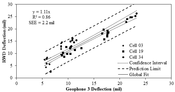
Figure 69 shows the overall plots obtained from the evaluation of the RWD. Overall, the RWD deflections were 11 percent greater than the embedded sensors. The figure also includes 95 percent confidence and prediction intervals. The confidence interval means that there is 95 percent probability that the population will lie within the confidence interval of the regression line calculated from the sample data. However, prediction interval is a range that is likely to contain the response value of a new observation given the linear regression model chosen.
1 mil = 0.0254 mm
Figure 69. Graph. Overall comparison of deflections measured with RWD and embedded sensors.
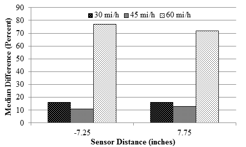
The impact of the vehicle speed on the performance of the RWD is demonstrated in figure 70. The y-axis corresponds to the median difference measured at all cells at a certain speed. Both sensors' median differences were higher when the RWD was operated at 60 mi/h (96.6 km/h) in comparison to the other two lower speeds.
1 mi/h = 1.61 km/h
1 inch = 25.4 mm
Figure 70. Graph. Median sensor difference for RWD with varying speeds.
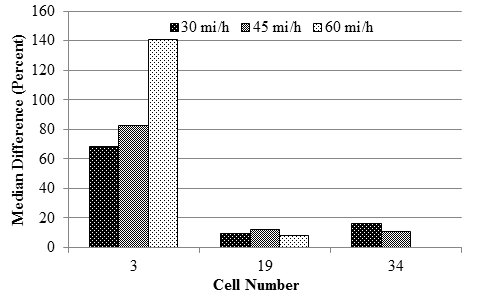
Cell stiffness seemed to impact the performance of the RWD as presented in figure 71. Sufficient data were not available to determine reason(s) for this impact. The stiffest section (cell 3) demonstrated a median difference ranging from 70 to 140 percent. Cell 19 had the smallest median difference of less than 10 percent for the three speeds. The median values minimized the uncertainties in the reported values related to occasional outliers observed during analysis.
1 mi/h = 1.61 km/h
Figure 71. Graph. Distributions of deflection difference measured with RWD for each cell.
TSD
As indicated, the parameter measured with a TSD is termed "deflection velocity" (i.e., particle velocity of the pavement surface). As such, a similar procedure as discussed for the RWD was followed to evaluate the TSD in terms of the deflection velocity. Table 24 depicts the overall results based on the deflection velocities and the two deflection estimation algorithms explained in section 5.6 (Data Analysis). The evaluation was limited to sensors that were 24 inches (609.6 mm) or less from the load since the deflections measured with the geophones and the TSD farther than that distance are considered to be too small to be sufficiently reliable.
| Parameter | Cell | Speed (mi/h) | Overall Statistics | ||||
|---|---|---|---|---|---|---|---|
| Constant (mil/s or mil)* | Slope | R2 Value | SEE (mil/s or mil)* | Average Deviation (Percent) | |||
| Velocity | 3 | 30 | 78.80 | 0.96 | 0.47 | 48.66 | 42 |
| 45 | 61.37 | 1.11 | 0.66 | 64.29 | 34 | ||
| 19 | 30 | 163.29 | 0.86 | 0.80 | 83.59 | 21 | |
| 45 | 109.10 | 0.94 | 0.97 | 44.88 | 9 | ||
| 60 | 97.26 | 0.97 | 0.93 | 89.16 | 7 | ||
| 34 | 30 | 225.83 | 0.81 | 0.92 | 90.32 | 6 | |
| 45 | 190.90 | 1.00 | 0.99 | 35.43 | 17 | ||
| Deflection method 1 | 3 | 30 | -1.90 | 0.97 | 0.85 | 0.91 | 22 |
| 45 | -2.52 | 1.02 | 0.90 | 0.73 | 25 | ||
| 19 | 30 | -2.71 | 1.05 | 0.93 | 1.39 | 11 | |
| 45 | -3.00 | 1.06 | 1.00 | 0.27 | 12 | ||
| 60 | -4.01 | 1.14 | 0.98 | 0.67 | 10 | ||
| 34 | 30 | -3.85 | 0.99 | 0.98 | 1.30 | 15 | |
| 45 | -7.81 | 1.17 | 0.99 | 0.70 | 13 | ||
| Deflection method 2 | 3 | 30 | 6.21 | 1.21 | 0.80 | 1.74 | 92 |
| 45 | 4.41 | 1.09 | 0.79 | 1.62 | 61 | ||
| 19 | 30 | 8.30 | 1.02 | 0.53 | 6.29 | 58 | |
| 45 | 9.21 | 1.04 | 0.96 | 1.35 | 65 | ||
| 60 | 3.61 | 0.87 | 0.74 | 3.26 | 12 | ||
| 34 | 30 | 3.04 | 0.97 | 0.98 | 1.54 | 9 | |
| 45 | 1.60 | 1.01 | 0.99 | 1.18 | 7 | ||
1 mi/h = 1.61 km/h
1 mil = 0.0254 mm
*Measured in mil/s for velocities and mil for deflections.
The constants from the best fit lines varied between 60 and 225 mil/s (1.5 and 5.7 mm/s). Given the narrow range, the difference may have been partially systematic, and hence it may have been possible to improve them with a more rigorous calibration of the device. For that reason, the constant values were considered systematic in the calculations of the differences. The slopes of the best fit lines varied between 0.81 and 1.11, which was fairly close to the ideal value of unity in most cases. The R2 values were reasonably close to unity except for the stiffest section (cell 3). The SEE values varied between 35 and 90 mil/s (0.9 and 2.3 mm/s), and they seemed to increase as the pavement became less stiff. Cell 3 also had the highest average deviation (over 34 percent). The average deviation for the less stiff cells (cells 19 and 34) was small, with the highest value being 17 percent. Up to 7 percent of these average deviations could be explained by the uncertainty of the data collection and analysis with the embedded sensors.
A review of the average deviations of the deflections indicates that method 1 was more appropriate for the data collected for this study. Even though method 2 provided more information about the deflection basins, it did not seem to represent the data from the three MnROAD cells as well.
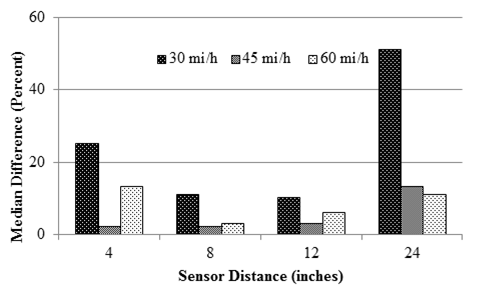
The average and standard deviation of differences of each individual sensor are presented in table 25. In terms of velocities, sensors located 4, 8, and 12 inches (101.6, 203.2, and 304.8 mm) away from the applied load seemed to match the embedded geophones' responses better with median differences of 13, 10, and 9 percent, respectively. Once again, the median values minimized the uncertainties in the reported values related to occasional outliers observed during analysis. The differences for sensors located farther than 24 inches (609.6 mm) from the applied load were in excess of 25 percent. In terms of the two methods proposed for the estimation of deflections, method 1 again seemed to be more representative of the MnROAD data.
| Parameter | Cell | Speed (mi/h) | Difference of Sensor at (Percent) | |||||||||
|---|---|---|---|---|---|---|---|---|---|---|---|---|
| 0 inches | 4 inches | 8 inches | 12 inches | 24 inches | ||||||||
| Mean Value | Standard Deviation | Mean Value | Standard Deviation | Mean Value | Standard Deviation | Mean Value | Standard Deviation | Mean Value | Standard Deviation | |||
| Velocity | 3 | 30 | NR | NR | 18 | 5 | 11 | 4 | 35 | 12 | 51 | 23 |
| 45 | NR | NR | 1 | 1 | 15 | 17 | 49 | 16 | 28 | 7 | ||
| 19 | 30 | NR | NR | 26 | 11 | 10 | 6 | 9 | 4 | 52 | 26 | |
| 45 | NR | NR | 12 | 1 | 2 | 2 | 2 | 1 | 13 | 10 | ||
| 60 | NR | NR | 13 | 5 | 3 | 3 | 6 | 6 | 11 | 11 | ||
| 34 | 30 | NR | NR | 25 | 10 | 16 | 10 | 10 | 11 | 45 | 9 | |
| 45 | NR | NR | 2 | 2 | 2 | 1 | 3 | 4 | 5 | 7 | ||
| Median | NR | NR | 13 | - | 10 | - | 9 | - | 28 | - | ||
| Deflection method 1 | 3 | 30 | 9 | 5 | NR | NR | 5 | 3 | 7 | 8 | NR | NR |
| 45 | 5 | 2 | NR | NR | 8 | 9 | 8 | 2 | NR | NR | ||
| 19 | 30 | 8 | 4 | NR | NR | 10 | 6 | 8 | 2 | NR | NR | |
| 45 | 6 | 2 | NR | NR | 7 | 2 | 5 | 2 | NR | NR | ||
| 60 | 14 | 3 | NR | NR | 18 | 4 | 11 | 5 | NR | NR | ||
| 34 | 30 | 1 | 1 | NR | NR | 7 | 1 | 8 | 2 | NR | NR | |
| 45 | 17 | 1 | NR | NR | 17 | 4 | 17 | 5 | NR | NR | ||
| Median | 8 | - | NR | NR | 8 | - | 8 | - | NR | NR | ||
| Deflection method 2 | 3 | 30 | 19 | 16 | 20 | 15 | 20 | 20 | 26 | 15 | 41 | 19 |
| 45 | 19 | 17 | 14 | 13 | 17 | 14 | 17 | 16 | 32 | 20 | ||
| 19 | 30 | 31 | 7 | 34 | 11 | 42 | 14 | 52 | 22 | 148 | 71 | |
| 45 | 15 | 7 | 6 | 6 | 7 | 6 | 9 | 9 | 37 | 13 | ||
| 60 | 14 | 7 | 13 | 14 | 17 | 20 | 22 | 18 | 79 | 72 | ||
| 34 | 30 | 10 | 2 | 4 | 4 | 7 | 3 | 7 | 6 | 23 | 17 | |
| 45 | 17 | 4 | 7 | 4 | 4 | 4 | 5 | 4 | 41 | 18 | ||
| Median | 19 | - | 14 | - | 18 | - | 21 | - | 34 | - | ||
1 mi/h = 1 km/h
1 inch = 25.4 mm
NR = Not reported.
- Indicates that the median was not calculated for the standard deviations.
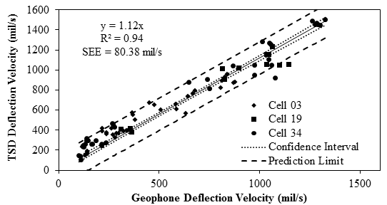
The TSD deflection velocities and estimated deflections from the two algorithms were compared with the corresponding deflection parameters from the embedded geophones in figure 72 through figure 74. The slope of the global fit depicted a difference of about 12 percent. The slope and an R2 value of 0.94 demonstrate the overall level of performance of the TSD. Most of the data points fall close to the global fit, generating a tight confidence interval and prediction limit with an SEE of about 80 mil/s (2.0 mm/s).
Sensors were also evaluated with varying vehicle speeds, and results are shown in figure 75. The median difference was the greatest for vehicle speeds of 30 mi/h (48.3 km/h) and usually the smallest at 45 mi/h (72.45 km/h).
1 mil/s = 0.0254 mm/s
Figure 72. Graph. Overall comparison of deflection velocities measured with TSD and embedded sensors.
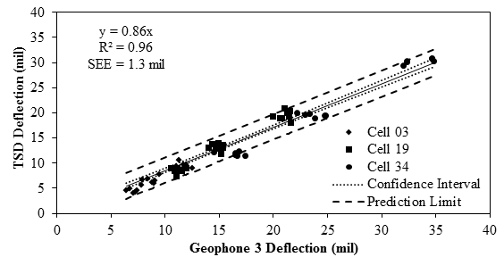
1 mil = 0.0254 mm
Figure 73. Graph. Overall comparison of TSD deflection method 1 and embedded sensors.
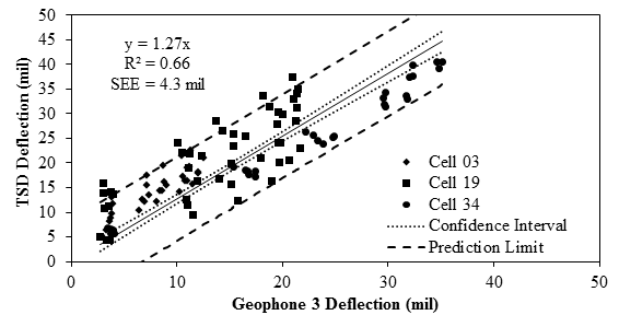
1 mil = 0.0254 mm
Figure 74. Graph. Overall comparison of TSD deflection method 2 and embedded sensors.
1 mi/h = 1.61 km/h
1 inch = 25.4 mm
Figure 75. Graph. Median sensor difference for TSD sensors with varying speeds.
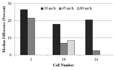
The variations in differences with pavement structure are summarized in figure 76. Median differences were obtained from all of the sensors' differences except for the one at 36 and 60 inches (914.4 and 1,524 mm). The stiffest cell (cell 3) had a median difference ranging from 22 to 27 percent at 30 and 45 mi/h (48.3 and 72.45 km/h). Cells 34 exhibited the lowest median difference (around 3 percent) at 45 mi/h (72.45 km/h).
1 mi/h = 1.61 km/h
Figure 76. Graph. Distribution of differences measured with TSD for each cell.
The evaluation of precision was carried out by analyzing the results obtained as discussed in section 5.6 (Data Analysis) for almost all MnROAD cells and the 18-mi (29-km) loop. To evaluate the influence of speed, temperature, and pavement structure and roughness in precision, each individual cell was also analyzed so that the variation in precision could be directly related to each of those factors. Several other factors such as the road geometry (slope and curves) were also studied less quantitatively using the 18-mi (29-km) loop data. Some other parameters such as the surface texture that are known to impact the precision could not be studied due to a lack of texture data. The results are discussed in the following subsection.
The RWD deflections were directly used for the precision analysis. However, the deflection slopes (i.e., deflection velocity divided by the vehicle speed) were used instead of the deflection velocity for the evaluation of TSD to reduce the speed-related variability in the results. The data from the TSD sensor placed 60 inches (1,524 mm) from the load were not considered in the precision analysis due to their high variability and small reported values.
Typical box plots, such as those shown in figure 63 through figure 66, were developed to delineate the median, upper, and lower quartiles and minimum and maximum values. The y-axis consisted of the slope, R2 value, SEE (as discussed in section 5.6, Data Analysis) and the range of measured values for all sections at all three speeds and during morning and afternoon. The precision of each sensor was evaluated individually.
RWD
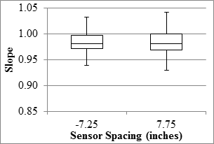
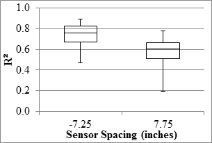
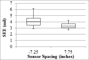
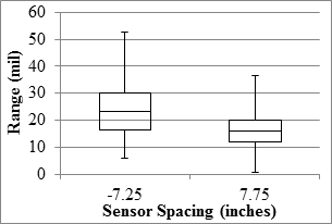
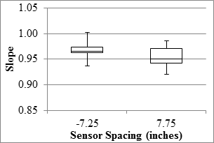
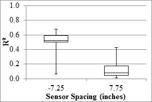
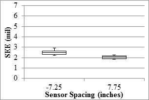
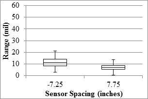
Overall results from the RWD along the MnROAD LVR and the mainline are presented in figure 77 through figure 84. The reported RWD data related to the PCC sections were limited to seven sections. As such, the results reported here are more relevant to the flexible and composite sections.
1 inch = 25.4 mm
Figure 77. Graph. RWD overall precision slope in the LVR.
1 inch = 25.4 mm
Figure 78. Graph. RWD overall precision R2 in the LVR.
1 mil = 0.0254 mm
1 inch = 25.4 mm
Figure 79. Graph. RWD overall precision SEE in the LVR.
1 mil = 0.0254 mm
1 inch = 25.4 mm
Figure 80. Graph. RWD overall precision range in the LVR.
1 inch = 25.4 mm
Figure 81. Graph. RWD overall precision slope in the mainline.
1 inch = 25.4 mm
Figure 82. Graph. RWD overall precision R2 in the mainline.
1 mil = 0.0254 mm
1 inch = 25.4 mm
Figure 83. Graph. RWD overall precision SEE in the mainline.
1 mil = 0.0254 mm
1 inch = 25.4 mm
Figure 84. Graph. RWD overall precision range in the mainline.
With slopes between the deflections from different passes averaging above 95 percent, both sensors exhibited satisfactory overall reproducibility. However, the median R2 values of 0.8 and lower indicate high scatter among deflections collected at each test point among different runs. The sensor located 7.25 inches (184.15 mm) behind the axle exhibited greater R2 values, especially along the LVR.
The median SEE from relating the deflections from different passes and sensors were 4 mil (0.1 mm) or less. The uncertainty of the measurements could be evaluated by comparing SEE with the range of deflections measured along the test sections. The median deflections were 24 mil (0.6 mm) or less for the sensor behind the axle and 16 mil (0.4 mm) or less for the sensor located 7.75 inches (196.85 mm) in front of the axle. As such, the median SEE was about 15 to 25 percent less than the median deflections measured by sensors.
Figure 85 through figure 88 depict the Wright County 18-mi (29-km) loop overall results, including the minimum, median, and maximum deflection parameters. The upper and lower quartiles are not shown because the experiments consisted of only three passes. Overall, the RWD exhibited a reasonable performance when tested under realistic environment. The slopes of the relationships among different passes typically yielded values equal or greater than 0.95 (i.e., close to the ideal value of unity). The R2 values were also above 0.86 for both sensors. The median SEE values were about 10 percent less than the median deflections for the sensor 7.25 inches (184.15 mm) behind and about 15 percent less than the sensor located 7.75 inches (196.85 mm) in front of the load. It should be mentioned that the data provided for the 18-mi (29-km) loop were averaged over 0.1 mi (0.161 km), whereas the data used in the precision and accuracy along the MnROAD were provided at 50-ft (15.25-m) intervals. This may explain the apparent higher precision of the RWD along the 18-mi (29-km) loop as compared to the MnROAD sections.
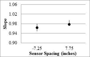
1 inch = 25.4 mm
Figure 85. Graph. RWD overall precision slope in the 18-mi (29-km) loop.
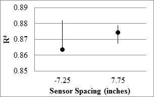
1 inch = 25.4 mm
Figure 86. Graph. RWD overall precision R2 in the 18-mi (29-km) loop.
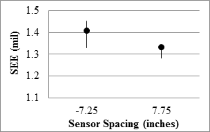
1 mil = 0.0254 mm
1 inch = 25.4 mm
Figure 87. Graph. RWD overall precision SEE in the 18-mi (29-km) loop.
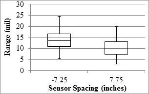
1 mil = 0.0254 mm
1 inch = 25.4 mm
Figure 88. Graph. RWD overall precision range in the 18-mi (29-km) loop.
TSD
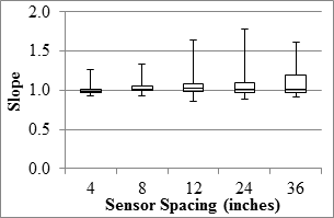
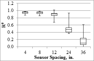
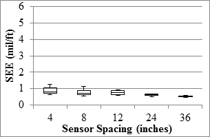
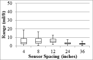
The TSD precision analyses were carried out based on deflection slopes and deflections estimated with the two methods discussed in section 5.6. Precision of the deflection slope varied with sensor spacing, as presented in figure 89 through figure 96. The median of the best fit slopes for all sensors was greater than 95 percent, indicating that the replicate data were in general agreement. The R2 values of the relationships between different passes were in excess of 0.9 for the first three sensors, indicating high certainty in the repeatability of the results from different passes. The farthest three sensors (including the sensor spaced 60 inches (1,524 mm) that is not shown here) yielded median R2 values that were less than desirable. A study by the manufacturer to assess the sources of the uncertainties of the last three sensors is warranted. The median SEE values were less than 1 mil/ft (0.08 mm/m) for the mainline sections and less than 2.5 mil/ft (0.20 mm/m) for the LVR sections. The repeatability of the sensor located at 36 inches (914.4 mm) might be of concern given that most of the measured deflection slopes were less than 3 mil/ft (0.08 mm/m).
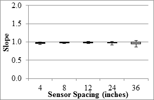
1 inch = 25.4 mm
Figure 89. Graph. TSD overall precision slope in the LVR.
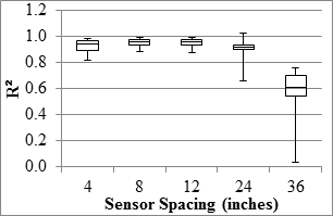
1 inch = 25.4 mm
Figure 90. Graph. TSD overall precision R2 in the LVR.
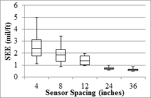
1 mil/ft = 83.3 µ/m
1 inch = 25.4 mm
Figure 91. Graph. TSD overall precision SEE in the LVR.
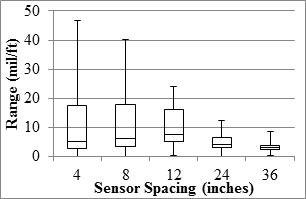
1 mil/ft = 83.3 µ/m
1 inch = 25.4 mm
Figure 92. Graph. TSD overall precision range in the LVR.
1 inch = 25.4 mm
Figure 93. Graph. TSD overall precision slope in the mainline.
1 inch = 25.4 mm
Figure 94. Graph. TSD overall precision R2 in the mainline.
1 mil/ft = 83.3 µ/m
1 inch = 25.4 mm
Figure 95. Graph. TSD overall precision SEE in the mainline.
1 mil/ft = 83.3 µ/m
1 inch = 25.4 mm
Figure 96. Graph. TSD overall precision range in the mainline.
Table 26 and table 27 contain the medians of the slope, R2, and SEE at different distances from the wheel's centerline. Both deflection algorithms estimated the deflection 0 inches (0 mm) from the centerline. For the available distances, both deflection methods resulted in an acceptable best fit slope. The median R2 and SEE values from deflection method 1 indicate a more precise method relative to method 2.
| Parameter | Test Section | Median Statistical Parameters | ||||||||
|---|---|---|---|---|---|---|---|---|---|---|
| 0 inches | 4 inches | 8 inches | ||||||||
| Slope | R2 | SEE | Slope | R2 | SEE | Slope | R2 | SEE | ||
| Deflection slope | LVR | NR | NR | NR | 0.97 | 0.95 | 2.40 | 0.98 | 0.96 | 1.86 |
| Mainline | NR | NR | NR | 0.99 | 0.96 | 0.81 | 1.01 | 0.95 | 0.73 | |
| 18-mi loop | NR | NR | NR | 0.93 | 0.71 | 1.31 | 0.96 | 0.78 | 1.11 | |
| Deflection method 1 | LVR | 0.99 | 0.95 | 2.23 | NR | NR | NR | 0.99 | 0.91 | 1.63 |
| Mainline | 1.02 | 0.82 | 1.35 | NR | NR | NR | 1.02 | 0.66 | 1.12 | |
| 18-mi loop | 0.98 | 0.81 | 1.87 | NR | NR | NR | 0.98 | 0.82 | 1.46 | |
| Deflection method 2 | LVR | 0.97 | 0.71 | 5.66 | 0.97 | 0.63 | 4.92 | 0.97 | 0.40 | 4.54 |
| Mainline | 1.03 | 0.16 | 4.68 | 1.03 | 0.30 | 4.42 | 1.03 | 0.46 | 4.13 | |
| 18-mi loop | 0.99 | 0.48 | 5.22 | 0.99 | 0.45 | 5.05 | 0.99 | 0.41 | 4.84 | |
1 inch = 25.4 mm
1 mi = 1.61 km
NR = Not reported.
| Parameter | Test Section | Median Statistic Parameters | |||||||||
|---|---|---|---|---|---|---|---|---|---|---|---|
| 12 inches | 24 inches | 36 inches | |||||||||
| Slope | R2 | SEE | Slope | R2 | SEE | Slope | R2 | SEE | |||
| Velocity | LVR | 0.99 | 0.96 | 1.35 | 0.98 | 0.92 | 0.70 | 0.98 | 0.61 | 0.60 | |
| Mainline | 1.02 | 0.91 | 0.76 | 1.01 | 0.47 | 0.63 | 1.02 | 0.10 | 0.52 | ||
| 18-mi loop | 0.95 | 0.79 | 1.00 | 0.99 | 0.80 | 0.65 | 1.01 | 0.72 | 0.59 | ||
| Deflection method 1 | LVR | 0.99 | 0.79 | 1.32 | - | - | - | - | - | - | |
| Mainline | 1.02 | 0.47 | 0.95 | - | - | - | - | - | - | ||
| 18-mi loop | 0.98 | 0.81 | 2.00 | - | - | - | - | - | - | ||
| Deflection method 2 | LVR | 0.96 | 0.19 | 4.15 | 0.93 | 0.24 | 3.87 | 0.89 | 0.29 | 3.66 | |
| Mainline | 1.02 | 0.49 | 3.97 | 1.00 | 0.48 | 3.84 | 0.97 | 0.49 | 3.57 | ||
| 18-mi loop | 0.99 | 0.35 | 4.65 | 0.97 | 0.09 | 4.30 | 0.94 | 0.15 | 3.90 | ||
1 inch = 25.4 mm
1 mi = 1.61 km
- Indicates that method 1 did not report these values.
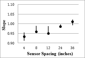
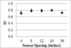
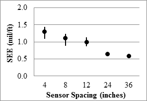
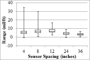
Figure 97 through figure 100 present the overall TSD results from the Wright County 18-mi (29-km) loop data averaged at a 33-ft (10 m) spacing. The precision of the TSD along the 18-mi (29-km) loop was similar or slightly worse in comparison to the MnROAD sections. The slopes of the best fit lines between repeat passes were greater than 0.92, but the R2 values were less than 0.8. The SEE gradually decreased from 1.3 to 0.6 mil/ft (0.11 to 0.05 mm/m), while the median range decreased from about 8 to 4 mil/ft (0.67 to 0.33 mm/m). Once again, the precision of the farther sensors was considered low.
1 inch = 25.4 mm
Figure 97. Graph. TSD overall precision slope in the 18-mi (29-km) loop.
1 inch = 25.4 mm
Figure 98. Graph. TSD overall precision R2 in the 18-mi (29-km) loop.
1 mil/ft = 83.3 µ/m
1 inch = 25.4 mm
Figure 99. Graph. TSD overall precision SEE in the 18-mi (29-km) loop.
1 mil/ft = 83.3 µ/m
1 inch = 25.4 mm
Figure 100. Graph. TSD overall precision range in the 18-mi (29-km) loop.
The stiffness of the pavement structure was defined using the average FWD deflection of the sensor directly under the load (center deflection) normalized to 11 kip (50 kN). MnROAD performs periodic FWD measurements. For this project, the FWD measurements at dates closest to the day of precision/accuracy testing were used. The precision of the device in each cell was also correlated to pavement roughness. The average IRI for each cell reported by the TSD during precision testing was used for this purpose. While the plots generated for this section were divided into flexible and rigid pavement, the trend lines corresponded to all sections.
TSDD precision for this and the following sections was evaluated using the median COVs of deflection parameters from each sensor within each cell. The COV of the deflection parameter from the three or five test repetitions at each individual data point within each cell was calculated. The median of these COV values was then extracted and used to avoid a statistical error from single marginal data point. For this section the median COVs from different times of day and different speeds were then averaged since this section only focuses on the correlation to pavement structure.
RWD
Figure 101 and figure 102 present the trends between the median coefficients of variation of deflection for each cell with the average FWD central deflection (as an indication of the structural stiffness of each cell). As the FWD deflection increased (i.e., the cell became structurally weaker), the COV of the RWD measurements decreased (i.e., the precision of the RWD increased). Based on limited accuracy data (see figure 71), the accuracy of the RWD measurements also decreased with an increase in stiffness.

1 mil = 0.0254 mm
1 inch = 25.4 mm
Figure 101. Graph. Comparison of RWD COV with pavement stiffness over flexible pavement.

1 mil = 0.0254 mm
1 inch = 25.4 mm
Figure 102. Graph. Comparison of RWD COV with pavement stiffness over rigid pavement.
Figure 103 and figure 104 depict the comparison between the RWD median COV of deflection and IRI. It is difficult to draw a conclusion on the influence of the IRI on the precision of the RWD given the scatter in the results.

1 inch/mi = 0.0158 m/km
1 inch = 25.4 mm
Figure 103. Graph. Comparison of RWD COV with IRI over flexible pavement.

1 inch/mi = 0.0158 m/km
1 inch = 25.4 mm
Figure 104. Graph. Comparison of RWD COV with IRI over rigid pavement.
TSD
Figure 105 and figure 106 depict the relationship between the median COV of the deflection slope for each cell and the average FWD deflection as a surrogate for the overall stiffness of the pavement structures. The spatial COVs associated with the first four sensors decreased as the FWD central deflection increased for the flexible pavements. The closest sensor exhibited higher COVs than the other sensors for the rigid pavements. From figure 76, the accuracy of the TSD for the flexible pavements was also impacted by the pavement stiffness. The median COVs of the deflection slopes are also correlated to the IRI measurements in figure 107 and figure 108. Once again, these two parameters are not strongly correlated.

1 mil = 0.0254 mm
1 inch = 25.4 mm
Figure 105. Graph. Precision TSD COV with pavement stiffness over flexible pavement.

1 mil = 0.0254 mm
1 inch = 25.4 mm
Figure 106. Graph. Precision TSD COV with pavement stiffness over rigid pavement.

1 inch/mi = 0.0158 m/km
1 inch = 25.4 mm
Figure 107. Graph. Precision TSD COV with IRI over flexible pavement.

1 inch/mi = 0.0158 m/km
1 inch = 25.4 mm
Figure 108. Graph. Precision TSD COV with IRI over rigid pavement.
To demonstrate the variation of the precision of the TSDDs with the vehicle speed, the median COVs of the deflection parameter from different passes within a cell of each sensor were calculated at different vehicle speeds as explained in the subsection, Correlation to Pavement Structure. The plots had to be separated between the MnROAD LVR and the mainline since the precision tests were carried out at different speeds along these two facilities. The LVR cells were tested at 30 and 45 mi/h (48.3 and 72.45 km/h), while the mainline tests were carried out at 45 and 60 mi/h (72.45 and 96.6 km/h). The common vehicle speed of 45 mi/h (72.45 km/h) was used as the common abscissa for reference.
RWD
Based on the slopes of the best fit lines shown in figure 109 and figure 110, the RWD became mildly (5 to 10 percent) less precise as the operational speed increased. The relationship shown in figure 109 for the LVR cells was stronger (i.e., exhibited higher R2 value) than the relationship from the mainline cells, as shown in figure 110. This trend could be attributed to the fact that the mainline cells were generally stiffer than the LVR cells. The RWD seemed to exhibit more precise measurements at lower speeds. Although measurements were not greatly affected by vehicle speed, the optimum operational speed should be the slowest one that is a compromise between operational costs and safety. Similar results were observed in figure 70 where the performance of the RWD was also negatively affected at a vehicle speed of 60 mi/h (96.6 km/h).

1 mi/h = 1.61 km/h
1 inch = 25.4 mm
Figure 109. Graph. Comparison of RWD COV at different speeds in the LVR.

1 mi/h = 1.61 km/h
1 inch = 25.4 mm
Figure 110. Graph. Comparison of RWD COV at different speeds in the mainline.
TSD
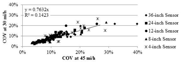
The relationships between the median COVs of the deflection slope at different vehicle speeds for the TSD are shown in figure 111 and figure 112. Although deflection slope was the parameter used for the TSD precision evaluation, the results appear to be affected by the vehicle speed. The COVs from tests at 30 mi/h (48.3 km/h) along the LVR were around 24 percent less than those measured at 45mi/h (72.45 km/h). The COVs from tests at 60 mi/h (96.6 km/h) were about 38 percent greater than the COVs measured at 45 mi/h (72.45 km/h) along the mainline.
1 mi/h = 1.61 km/h
1 inch = 25.4 mm
Figure 111. Graph. Comparison of TSD COV at different speeds in the LVR.

1 mi/h = 1.61 km/h
1 inch = 25.4 mm
Figure 112. Graph. Comparison of TSD COV at different speeds in the mainline.
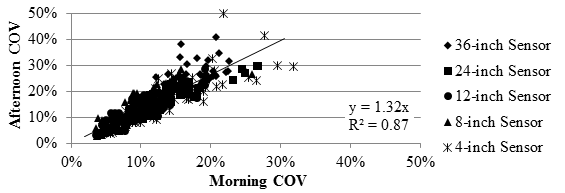
The same procedure followed for vehicle speed was used to estimate the impact of temperature variation on the precision of the TSDDs. Similar plots were developed to compare the median COVs of deflection slopes from morning runs with those from afternoon runs. Table 28 includes the average and COVs of the pavement temperature during precision testing as measured by both TSDDs.
| Test Section | Morning Temperature | Afternoon Temperature | ||
|---|---|---|---|---|
| Average (°F) | COV (Percent) | Average (°F) | COV (Percent) | |
| LVR | 68 | 6.4 | 92 | 5.2 |
| Mainline | 80 | 9.1 | 92 | 5.4 |
1 °F = 1.8 °C + 32
RWD
RWD results are presented in figure 113. A weak correlation between the afternoon and morning COVs of the deflections could be observed considering that the R2 value was 0.61. Afternoon runs were around 7 percent more precise than morning runs. One reason for this pattern could be that high temperatures create a softer surface layer that increases the measured deflections. For the same sensors, higher precision is expected as the measured parameter increases. RWD consistently showed lower precision when the measured deflections were small for stiffer pavement or when the device was operated at higher vehicle speed.

1 inch = 25.4 mm
Figure 113. Graph. Comparison of RWD COV at different afternoon temperatures.
TSD
Change in pavement temperature affected the TSD differently. The precision of the TSD, presented in figure 114, seemed to decrease with higher temperatures. Afternoon runs yielded COVs that were 32 percent greater than the measurements in the morning. With an R2 value of 0.87, the precisions from the morning and afternoon tests were more correlated than from the RWD.
1 inch = 25.4 mm
Figure 114. Graph. Comparison of TSD COV at different afternoon temperatures.
Vertical and Horizontal Curves
The impact of the vertical gradient and horizontal curves on the precision of the TSD was studied only for the 18-mi (29-km) loop using the data reported at 33-ft (10-m) intervals. Such analysis was not feasible for the RWD because the data were reported every 0.1 mi (0.161 km). Enough data were not available to carry out a conclusive study with the RWD.
Correlation to Vertical Gradient
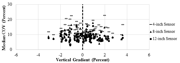
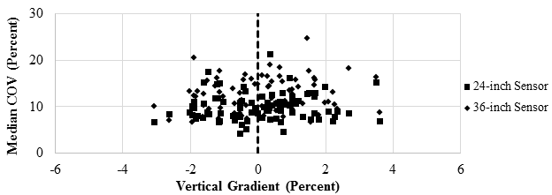
The 18-mi (29-km) loop was first divided into 0.2-mi (0.322-km) increments. The vertical gradient of the road was estimated for each subsection by dividing the change in elevation as measured by the TSD by the horizontal distance (0.2 mi (0.322 km)). The median COV within each increment was determined and plotted against the vertical gradient. Figure 115 and figure 116 detail the results from the five closest sensors for the TSD. A zero elevation change was denoted with a dashed line, delineating the downhill sections from uphill sections. No clear correlation related to a vertical gradient was found.
1 inch = 25.4 mm
Figure 115. Graph. Precision TSD COV with vertical gradients for the closer sensors.
1 inch = 25.4 mm
Figure 116. Graph. Precision TSD COV with vertical gradients for the further sensors.
Correlation to Horizontal Curves
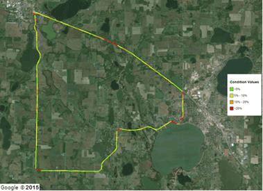
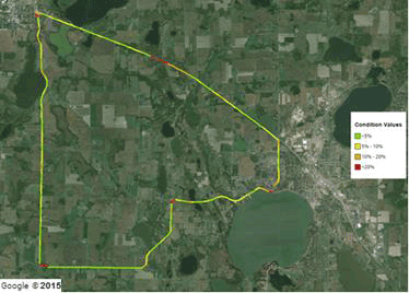
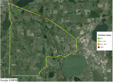
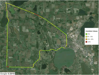
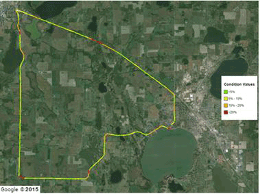
Google© maps of the COVs of the deflection slopes from repeated runs for the first five sensors are shown in figure 117 through figure 121. Qualitatively, most of the relatively high COVs (i.e., red and orange sections) correspond to sharp turns and/or locations of the stop signs.
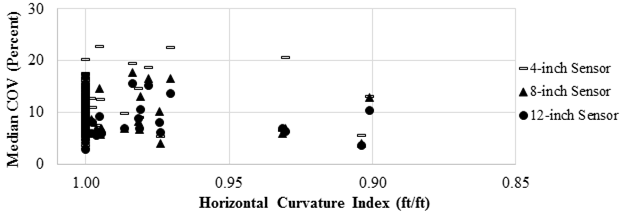
In order to quantify the horizontal curvature of the road, the horizontal curvature index was obtained for each 0.2-mi (0.322-km) subsection. This index was approximated using the GPS coordinates. The horizontal curvature index was estimated by dividing the straight distance between the beginning and ending of each subsection by the total traveled distance between those two points. A straight section of the road would result in a horizontal curvature index of unity since the direct distance and the traveled distance are the same. The smaller the curvature index, the curvier the 0.2-mi (0.322-km) subsection will be. Figure 122 and figure 123 depict the correlation between the median COV of the TSD measurements and the horizontal curvature index of the subsections. Most subsections in the 18-mi (29-km) loop constituted straight roads denoted by value of 1. A clear correlation was not present in the plot. All subsections including those with sharp horizontal curvatures resulted in a COV ranging between 5 and 25 percent.
©2015 Google® (Modifications: See Acknowledgements).
Figure 117. Map. Wright County 18-mi (29-km) loop TSD 36-inch (914.4-mm) sensor COV.(46)
©2015 Google® (Modifications: See Acknowledgements).
Figure 118. Map. Wright County 18-mi (29-km) loop TSD 24-inch (609.6-mm) sensor COV.(47)
©2015 Google® (Modifications: See Acknowledgements).
Figure 119. Map. Wright County 18-mi (29-km) loop TSD 12-inch (304.8-mm) sensor COV.(48)
©2015 Google® (Modifications: See Acknowledgements).
Figure 120. Map. Wright County 18-mi (29-km) loop TSD 8-inch (203.2-mm) sensor COV.(49)
©2015 Google® (Modifications: See Acknowledgements).
Figure 121. Map. Wright County 18-mi (29-km) loop TSD 4-inch (101.6-mm) sensor COV.(50)
1 ft/ft = 1 m/m
1 inch = 25.4 mm
Figure 122. Graph. Precision TSD COV with horizontal curves for the closer sensors.

1 ft/ft = 1 m/m
1 inch = 25.4 mm
Figure 123. Graph. Precision TSD COV with horizontal curves for the further sensors.
This chapter includes the overall evaluation of the RWD and TSD. The performance of both TSDDs varied under different conditions. Based on the results of the analyses presented in this chapter, it was found that both devices were capable of providing reasonably accurate and precise pavement response measurements. The information presented in this chapter can also be used to recommend the optimum operational conditions and to identify device limitations, both of which are addressed in chapter 10 of this report. Conclusions and recommendations within this chapter were limited by the amount of data available for this project.