Pavement Structural Evaluation at the Network Level: Final Report

 

CHAPTER 8. DEFLECTION BASIN INDICES

8.1. Introduction

This chapter presents details concerning the analytical investigation undertaken to explore relationships between load-induced structural-related responses of a pavement system and the corresponding surface deflection basin-related indices. This investigation and associated results were considered an important effort toward the development of methodologies for incorporating TSDD measurements into network-level PMS applications.

Pavement failure (or structural capacity), in terms of fatigue or rutting can be estimated from performance prediction equations.^(27,57) These equations relate load-induced pavement responses to the following two important pavement distresses: (1) certain level of AC fatigue cracking and (2) rutting failure in the subgrade. The critical load-induced pavement responses that relate to the two referenced distresses are the maximum tensile horizontal strain (also known as fatigue strain) at the bottom of the AC layer and the vertical compressive strain on top of the subgrade, respectively. In addition, there are studies that postulate the existence of reliable correlations between deflection basin- related indices and load-induced pavement structural responses, which suggest it is possible to correlate deflection basin indices to structural capacity (or distress).^(62,63,21)

Specific TSDD deflection basin measurements depend on the device under consideration. For example, the TSD device measures surface vertical velocity at as many as nine locations within the deflection bowl, and subsequently, the surface vertical deflection basin is determined based on a certain assumption for the shape of the defection basin. Conversely, only two surface measurements within the deflection bowl are taken by the RWD. In turn, this means that the selection of deflection basin indices for correlation to structural capacity (or distress) must take into consideration the capabilities of the specific TSDD.

Chapter 7 of this report detailed the validation of the 3D-Move program, for the purposes of the project in question, using a variety of independent pavement responses that included surface deflection bowls (measured using project sensors) as well as horizontal strains at the bottom of the AC layers and vertical stresses at the top of the subgrade (measured using MnROAD sensors). Accordingly, the program was ready for the evaluation of the critical pavement responses and corresponding deflection-based indices, thus enabling the investigation of correlations between the two. Because 3D-Move uses a dynamic moving load model, important factors such as viscoelastic properties and vehicle speed can be accounted for in the evaluation of pavement response time histories.

A number of previous studies have proposed many surface vertical deflection-based indices, and they have also postulated that these indices relate to the structural capacity of pavements.^(62,63,21) However, for the purposes of this project, it was important to identify those indices that best relate to the two critical pavement responses. The identification of the appropriate indices was undertaken using the following three-step procedure:

1. Step 1: Identified the surface deflection indices that correlated well with the critical pavement responses using the 3D-Move simulation results presented in chapter 7, which were based on the TSDD field trials carried out at the MnROAD facility.
   
   
2. Step 2: Used a set of 36 pavement structures (different combinations of layer thicknesses and moduli) and vehicle speed combinations (hereafter referred to as combinations) as input to 3D-Move to perform a sensitivity analysis of the correlations associated with various deflection indices (not limited to those indices identified in step 1).
   
   
3. Step 3: Used the JULEA layered elastic program to further explore the robustness of the correlations identified in the first two steps by considering a much larger database (approximately 15,000 different pavement combinations) of pavements.⁽²⁶⁾ There were limitations (e.g., stationary, static, and elastic) associated with JULEA relative to realistic modeling of pavement response. However, if narrowly constrained correlations irrespective of pavement material properties were found through the use of the large JULEA database, then the impact of these limitations may not have been significant.
   
   

These three steps used to identify the most appropriate indices are described in greater detail in the following subsections.

8.2 Step 1: Using Existing 3D-Move Simulation Results

As a part of the calibration process described in chapter 7, pavement responses using 3D-Move were computed for three MnROAD accuracy cells with the TSDDs travelling at various vehicle speeds. By trial and error, three pavement case scenarios were identified for each of the accuracy cells, which bracketed the vertical surface deflection bowls computed by 3D-Move with those measured by the project sensors. In all, 42 datasets of pavement responses and corresponding vertical surface deflections datasets were generated using 3D-Move.

Defining Response Points in 3D-Move Runs

The 3D-Move program can output many response time histories (e.g., stresses, strains, displacements, and velocities) as a vehicle travels on at any specified location of the pavement surface. The TSDDs measured (or estimated) vertical surface deflections at many predetermined locations in the longitudinal direction along the midline between the rear tires (see figure 166). From the vertical displacement time history computed by 3D-Move at a point (observation point) on the midline between the tires, it was possible to determine the displacements at various individual locations along the midline using time space superposition. The 3D-Move output includes the time of the maximum displacement (t_max) and also the time (t_o) at which the instantaneous deflection at the midpoint between tires (D₀) reached the point of observation (see figure 167). Since 3D-Move modeled the damping characteristics of the pavement layers, there was an offset between t_max and t_o. The location D_r refers to a point at a distance r in inches in front of D₀. The maximum displacement that occurred at the location D_max and other displacements at many locations shown along the midline between the tires in figure 166 could be readily determined using time-space superposition.

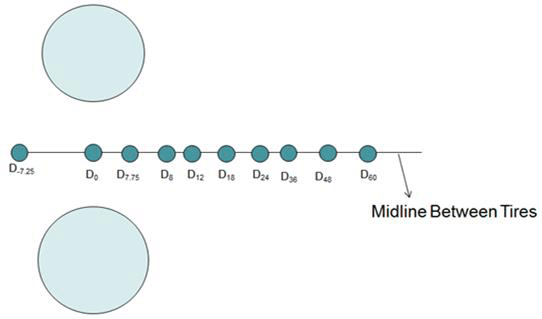
Figure 166. Illustration. Predetermined locations for estimation of vertical surface deflections in TSDDs.

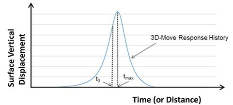
Figure 167. Illustration. Surface displacement from 3D-Move displacement time history.

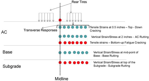
Conversely, when other 3D-Move pavement responses (e.g., maximum AC tensile strain) were considered, it was necessary to select multiple transverse locations (the depth was fixed) in the computations. This is because the location of the maximum value of the response was not known a priori. After computing responses at many multiple transverse locations, the maximum response value could be determined.

Though the focus of this project was on the horizontal (or fatigue) strains at the bottom the AC and to a lesser extent on the vertical strains at the top of subgrade, a larger database of pavement responses was assembled from the 3D-Move runs. The list of the locations and corresponding responses and the distress mode includes the following (see figure 168):

• Bottom of AC tensile strains in x and y direction for bottom-up fatigue cracking.
  
  
• Tensile strains at surface and 0.5 inch (12.7 mm) from surface of AC for top-down cracking.
  
  
• Vertical strain/stress 2 inches (50.8 mm) from AC surface for rutting estimate of AC.
  
  
• Vertical stress/strain at mid-point of base for base rutting.
  
  
• Vertical strains on top of the subgrade for subgrade rutting.

1 inch = 25.4 mm

Figure 168. Illustration. Selection of response points when using 3D-Move.

Pavement Properties and Loading in 3D-Move Runs

The initial focus of the simulations was on the three MnROAD cells (cells 3, 19, and 34), where project sensor measurements were taken during the TSDD field trials. A sketch of the pavement structures at these three cells was presented earlier in figure 141 (see chapter 7). Since the AC thickness varied from 3 to 5 inches (76.2 to 127 mm) along these cells, the sections could be categorized as pavements with relatively thin AC. Other pavement layer thicknesses and moduli are also shown in this figure. To compare the 3D-Move results to measured data from the MnROAD and project sensors, the AC moduli corresponding to the temperatures at the time of the TSDD field trials were required. The procedure to get the AC layer modulus versus frequency relation at any given temperature based on FWD backcalculated layer moduli was described in chapter 7. Figure 138 and figure 139 in chapter 7 showed the axle configuration and loads for the TSD and RWD. These two cases of loading (tire loads, pressure, and spacing) could be used to determine the role of loading conditions on the correlations between surface deflection indices and pavement responses as described later in this chapter.

Selection of Deflection Basin Indices

A number of deflection basin-related indices have been proposed by researchers and are perceived as strong predictors of the critical structural-related responses and structural conditions (or capacity) of the pavements. Experimental and analytical studies have reported strong correlations between some deflection basin indices and pavement responses.^(62,63,21) Horak proposed two different equations for R referred as R1 and R2 as in Figure 8 and Figure 9.^(63,64)

As noted previously, the 3D-Move deflection basin parameters were computed based on surface vertical displacement along the midline between the two rear tires, while the maximum pavement responses were determined by considering many transverse response locations. The 3D-Move runs initially used both the TSD and RWD loadings individually, and then the combined dataset were used when exploring the correlations. A power curve generally described the data better than a linear fit, as judged by improved correlation coefficients (R²).

SCI is typically defined as the difference in displacements between D₀ and D_r. D₀ is the reference displacement; however, the locations D₀ and D_max were not the same due to viscous lag of the response due to the moving load. Accordingly, it was important to determine whether a better correlation existed if D_max was used as the reference displacement. Parameter SCIm is defined by using D_max instead of D₀ as the reference displacement in the calculations of the indices. Since both TSD and RWD did not directly measure deflection at D₀, another observation made during the investigation was the need to also consider D₄, D_-7.25, and D₈ (i.e., displacements at 4, -7.25, and 8 inches (101.6, -184.15, and 203.2 mm), respectively) as reference displacement locations. In the case of the TSD, because of its capacity to measure multiple deflection points, a theoretical algorithm was used to compute D₀. However, to minimize additional computations and associated errors, the possibility of utilizing direct TSD measurements at D₄ and D₈ were proposed. More specifically, a new index called Deflection Slope Index (DSI) was proposed based on reference at D₄, D₈, D₁₂, D₁₈, and D₂₄. DSI is the difference between the deflection at reference location and D_r. In addition, indices representing deflection slope at a given location defined as Tangent Slope (TS) was also considered.

Table 44 shows these indices. A total of 75 individual indices are listed in this table. The deflection basin indices included in table 44 correlated with the two pavement structural-related responses presented earlier in this chapter. The deflection basin parameters that did not yield strong correlations to the structural-related responses were not considered further under the third step.

Table 44. Deflection basin indices used in the evaluation.

Parameter and Number of Indices	Indices for Evaluation
R1 (7)	R18
	R112
	R118
	R124
	R136
	R148
	R160
R2 (7)	R28
	R212
	R218
	R224
	R236
	R248
	R260
Surface displacement (2)	D0
	D60
Area (1)	A
Shape factors (2)	F1
	F2
SCI (7)	SCI8
	SCI12
	SCI18
	SCI24
	SCI36
	SCI48
	SCI60
	D-7.25 - D7.75 (for RWD)
BCI (1)	BCI
BDI (1)	BDI
AUPP (1)	AUPP
SD (7)	SD8
	SD12
	SD18
	SD24
	SD36
	SD48
	SD60
TS (8)	TS4*
	TS8*
	TS12*
	TS18
	TS24*
	TS36*
	TS48
	TS60*
SCIm (7)	SCIm8
	SCIm12
	SCIm18
	SCIm24
	SCIm36
	SCIm48
	SCIm60
DSI4-r (7)	DSI4 - 8
	DSI4 - 12
	DSI4 - 18
	DSI4 - 24
	DSI4 - 36
	DSI4 - 48
	DSI4 - 60
DSI8 - r (6)	DSI8 - 12
	DSI8 - 18
	DSI8 - 24
	DSI8 - 36
	DSI8 - 48
	DSI8 - 60
DSI12 - r (4)	DSI12 - 18
	DSI12 - 24 (same as BDI)
	DSI12 - 36
	DSI12 - 48
	DSI12 - 60
DSI18 - r (4)	DSI18 - 24
	DSI18 - 36
	DSI18 - 48
	DSI18 - 60
DSI24 - r (2)	DSI24 - 36 (same as BCI)
	DSI24 - 48
	DSI24 - 60

*TSD sensor location.

Note: Numbers within parentheses in left column indicate the number of indices for each deflection basin parameter.

The goodness of the correlations between the indices and pavement responses were categorized into three classes. Class 1 indices had an R² greater than 0.9 and were considered the most appropriate indices. Class 2 indices were those with an R² between 0.7 and 0.9, and class 3 indices were those with an R² less than 0.7.

Two options were used when horizontal strains at the bottom AC were considered: (1) maximum tensile strains in transverse and longitudinal direction of vehicle travel and (2) maximum tensile strains at a location directly below the midpoint between the rear tires. For the purpose of brevity, only the following tables and figures that showed the highest (and therefore the most appropriate) correlations are included in this chapter:

• Table 45, table 46, figure 169, and figure 170 show the relationships with R1 shown in table 44.
  
  
• Table 47, table 48, figure 171, and figure 172 show the relationships with SCI, where D₀ was used as the reference displacement.
  
  
• Table 49, table 50, figure 173, and figure 174 show the relationships with SCIm, where D_max was used as the reference displacement.
  
  
• Table 51, table 52, figure 175, and figure 176 show the relationships with DSI, where D₄ was used as the reference displacement.

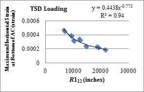
The equations with R² values more than 0.90 are presented bold. The example tables and figures provide results for TSD loadings only and also for the combined TSD and RWD loadings. There are 17 data points available for the TSD loadings and 43 for the combined dataset. Similar tables and figures looking at the fatigue strain relationship were developed for every index in table 44, but they are not included in the report, as they do not provide further insights. The data used to generate these tables and figures can be obtained directly from FHWA.

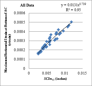
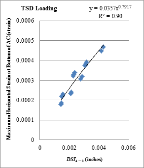
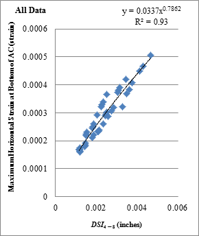
Based on the information presented in table 45 through table 52 and the review of the correlations for other indices, it was concluded that indices based on maximum horizontal strains were better than horizontal strains at the location directly below the midpoint between the tires. It was also concluded that the role of the difference in load characteristics (TSD versus RWD) on the relationships were minimal. However, SCIm, which used D_max as the reference displacement, had a slightly better correlation. It also appears that using D₄ instead of D₀ to calculate SCI yielded better correlations.

Table 45. Relationships between R1 and horizontal strains at bottom of AC with TSD loading data.

Index	Relation with Midline Horizontal Strain*		Relation with Maximum Horizontal Strain*
	Equation	R2	Equation	R2
R18	y = 3.3238x-1.02	0.75	y = 1.2327x-0.896	0.88
R112	y = 1.3707x-0.912	0.85	y = 0.4438x-0.775	0.94
R118	y = 0.5819x-0.791	0.88	y = 0.1802x-0.655	0.92
R124	y = 0.4157x-0.73	0.88	y = 0.1241x-0.595	0.89
R136	y = 0.397x-0.684	0.87	y = 0.1115x-0.551	0.86
R148	y = 0.5396x-0.682	0.87	y = 0.1395x-0.547	0.85
R160	y = 0.7837x-0.69	0.87	y = 0.1866x-0.553	0.85

*At the bottom of AC layer.

y = Horizontal strain.

x = Index.

Note: There were 17 TSD loading data points. Bold cells indicate indices in class 1.

Table 46. Relationship between R1 and horizontal strains at bottom of AC with all loading data.

Index	Relation with Midline Horizontal Strain*		Relation with Maximum Horizontal Strain*
	Equation	R2	Equation	R2
R18	y = 6.2386x-1.091	0.74	y = 1.2078x-0.895	0.88
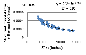
R112	y = 2.2986x-0.968	0.87	y = 0.3945x-0.763	0.95
R118	y = 0.9436x-0.843	0.91	y = 0.1584x-0.643	0.93
R124	y = 0.6542x-0.778	0.91	y = 0.1079x-0.583	0.90
R136	y = 0.6504x-0.733	0.90	y = 0.0994x-0.542	0.87
R148	y = 0.9188x-0.732	0.89	y = 0.125x-0.539	0.85
R160	y = 1.3733x-0.742	0.89	y = 0.1666x-0.545	0.85

*At the bottom of AC layer.

y = Horizontal strain.

x = Index.

Note: There were 43 data points from both TSD and RWD loading. Bold cells indicate indices in class 1.

1 inch = 25.4 mm

Figure 169. Graph. Relationship between R1₁₂ and horizontal strains at bottom of AC with TSD loading data.

1 inch = 25.4 mm

Figure 170. Graph. Relationship between R1₁₂ and horizontal strains at bottom of AC with all loading data.

Table 47. Relationship between SCI and horizontal strains at bottom of AC with TSD loading data.

Index	Relation with Midline Horizontal Strain*		Relation with Maximum Horizontal Strain*
	Equation	R2	Equation	R2
SCI8	y = 0.0969x1.0201	0.75	y = 0.0553x0.8958	0.88
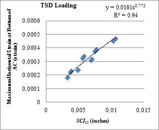
SCI12	y = 0.0277x0.9119	0.85	y = 0.0161x0.775	0.94
SCI18	y = 0.0104x0.7911	0.88	y = 0.0064x0.6547	0.92
SCI24	y = 0.0067x0.73	0.88	y = 0.0043x0.5948	0.89
SCI36	y = 0.0047x0.6841	0.87	y = 0.0031x0.551	0.86
SCI48	y = 0.0044x0.6817	0.87	y = 0.003x0.547	0.85

*At the bottom of AC layer.

y = Horizontal strain.

x = Index.

Note: There were 17 TSD loading data points. Bold cells indicate indices in class 1.

Table 48. Relationship between SCI and horizontal strains at bottom of AC with all loading data.

Index	Relation with Midline Horizontal Strain*		Relation with Maximum Horizontal Strain*
	Equation	R2	Equation	R2
SCI8	y = 0.142x1.0914	0.74	y = 0.0543x0.8949	0.88
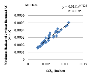
SCI12	y = 0.0365x0.9684	0.87	y = 0.0151x0.7626	0.95
SCI18	y = 0.0129x0.8432	0.91	y = 0.006x0.6427	0.93
SCI24	y = 0.008x0.778	0.91	y = 0.004x0.5827	0.90
SCI36	y = 0.0056x0.7335	0.90	y = 0.003x0.5422	0.86
SCI48	y = 0.0053x0.7324	0.89	y = 0.0028x0.5392	0.85

*At the bottom of AC layer.

y = Horizontal strain.

x = Index.

Note: There were 43 data points from both TSD and RWD loading. Bold cells indicate indices in class 1.

1 inch = 25.4 mm

Figure 171. Graph. Relationship between SCI₁₂ and horizontal strains at bottom of AC with TSD loading data.

1 inch = 25.4 mm

Figure 172. Graph. Relationship between SCI₁₂ and horizontal strains at bottom of AC with all loading data.

Table 49. Relationship between SCIm and horizontal strains at bottom of AC with TSD loading data.

Index	Relation with Midline Horizontal Strain*		Relation with Maximum Horizontal Strain*
	Equation	R2	Equation	R2
SCIm8	y = 0.0713x0.9751	0.76	y = 0.0417x0.854	0.89
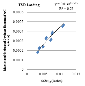
SCIm12	y = 0.0234x0.883	0.84	y = 0.014x0.7505	0.92
SCIm18	y = 0.0096x0.7774	0.88	y = 0.0061x0.6437	0.92
SCIm24	y = 0.0063x0.7211	0.87	y = 0.0041x0.5879	0.89
SCIm36	y = 0.0046x0.6782	0.87	y = 0.0031x0.5465	0.86
SCIm48	y = 0.0043x0.6763	0.86	y = 0.0029x0.5429	0.85

*At the bottom of AC layer.

y = Horizontal strain.

x = Index.

Note: There were 17 TSD loading data points. Bold cells indicate indices in class 1.

Table 50. Relationship between SCIm and horizontal strains at bottom of AC with all loading data.

Index	Relation with Midline Horizontal Strain*		Relation with Maximum Horizontal Strain*
	Equation	R2	Equation	R2
SCIm8	y = 0.1022x1.0439	0.77	y = 0.0407x0.8526	0.91
SCIm12	y = 0.0306x0.9386	0.87	y = 0.0131x0.739	0.95
SCIm18	y = 0.012x0.8292	0.91	y = 0.0057x0.6323	0.93
SCIm24	y = 0.0076x0.7689	0.91	y = 0.0038x0.5763	0.89
SCIm36	y = 0.0055x0.7274	0.90	y = 0.0029x0.538	0.86
SCIm48	y = 0.0051x0.7268	0.89	y = 0.0027x0.5354	0.85

*At the bottom of AC layer.

y = Horizontal strain.

x = Index.

Note: There were 43 data points from both TSD and RWD loading. Bold cells indicate indices in class 1.

1 inch = 25.4 mm

Figure 173. Graph. Relationship between SCIm₁₂ and horizontal strains at bottom of AC with TSD loading data.

1 inch = 25.4 mm

Figure 174. Graph. Relationship between SCIm₁₂ and horizontal strains at bottom of AC with all loading data.

Table 51. Relationship between DSI_{4 - r} and horizontal strains at bottom of AC with TSD loading data.

Index	Relation with Midline Horizontal Strain*		Relation with Maximum Horizontal Strain*
	Equation	R2	Equation	R2
DSI4 - 8	y = 0.0641x0.9153	0.79	y = 0.0357x0.7917	0.90
DSI4 - 12	y = 0.0201x0.8324	0.84	y = 0.0119x0.7019	0.91
DSI4 - 18	y = 0.0086x0.7386	0.87	y = 0.0054x0.6079	0.90
DSI4 - 24	y = 0.0057x0.6872	0.87	y = 0.0037x0.5573	0.87

*At the bottom of AC layer.

y = Horizontal strain.

x = Index.

Note: There were 17 TSD loading data points. Bold cells indicate indices in class 1.

Table 52. Relationship between DSI_{4 - r} and horizontal strains at bottom of AC with all loading data.

Index	Relation with Midline Horizontal Strain*		Relation with Maximum Horizontal Strain*
	Equation	R2	Equation	R2
DSI4 - 8	y = 0.0891x0.9776	0.82	y = 0.0337x0.7862	0.93
DSI4 - 12	y = 0.0257x0.8833	0.88	y = 0.0111x0.6886	0.94
DSI4 - 18	y = 0.0104x0.7857	0.91	y = 0.005x0.5947	0.91
DSI4 - 24	y = 0.0067x0.7313	0.90	y = 0.0035x0.5445	0.88

*At the bottom of AC layer.

y = Horizontal strain.

x = Index.

Note: There were 43 data points from both TSD and RWD loading. Bold cells indicate indices in class 1.

1 inch = 25.4 mm

Figure 175. Graph. Relationship between DSI_{4 - 8} and horizontal strains at bottom of AC with TSD loading data.

1 inch = 25.4 mm

Figure 176. Graph. Relationship between DSI_{4 - 8} and horizontal strains at bottom of AC with all loading data.

Because vertical strain at the top of the subgrade is an important response that relates to subgrade rutting, the deflection basin indices considered were also correlated with those strains.

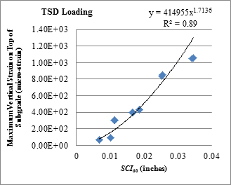
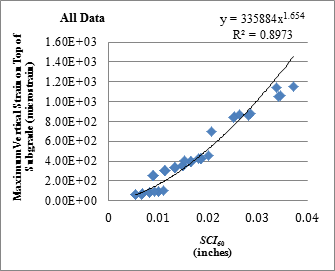
Table 53, table 54, figure 177, and figure 178 show the relationships between SCI and vertical strain at the top of the subgrade. While SCI (e.g., SCI₁₂) was one of the most appropriate indices related to maximum horizontal strain at the bottom of AC, it cannot be used to relate to subgrade strain because of poor correlation.

Table 53. Relationship between SCI and maximum vertical strains on top of the subgrade with TSD loading data.

Index	Relation with Maximum Vertical Strain*
	Equation	R2
SCI8	y = 1E+07x1.7785	0.38
SCI12	y = 6E+06x1.904	0.62
SCI18	y = 2E+06x1.7981	0.76
SCI24	y = 815968x1.7374	0.84
SCI36	y = 447767x1.6776	0.88
SCI48	y = 402727x1.6869	0.89
SCI60	y = 414955x1.7136	0.89

*On top of subgrade.

y = Vertical strain.

x = Index.

Note: There were 17 TSD loading data points.

Table 54. Relationship between SCI and maximum vertical strains on top of the subgrade with all loading data.

Index	Relation with Maximum Vertical Strain*
	Equation	R2
SCI8	y = 9E+06x1.752	0.39
SCI12	y = 4E+06x1.8178	0.62
SCI18	y = 1E+06x1.7333	0.78
SCI24	y = 621344x1.6678	0.84
SCI36	y = 360860x1.6188	0.88
SCI48	y = 328608x1.63	0.89
SCI60	y = 335884x1.654	0.90

*On top of subgrade.

y = Vertical strain.

x = Index.

Note: There were 43 data points from both TSD and RWD loading. Bold cells indicate indices in class 1.

1 inch = 25.4 mm

Figure 177. Graph. Relationship between SCI₆₀ and maximum vertical strain on top of the subgrade with TSD loading data.

1 inch = 25.4 mm

Figure 178. Graph. Relationship between SCI₆₀ and maximum vertical strain on top of the subgrade with all loading data.

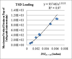
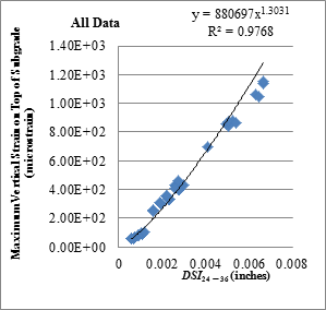
Table 55, table 56, figure 179, and figure 180 show the relationships between DSI_{24 - r} and vertical strain at the top of the subgrade. DSI_{24 - 36}, which is also known as BCI, had a good correlation, indicated by class 1 classification. Moreover, it was observed that those indices based on displacements at far away locations from the loaded area were better related to vertical strain at the top of the subgrade. This is because these indices reflect the influence of the lower portion of the pavement system.^(62,63) Similar tables and figures looking at the rutting strain relationship were developed for every index in table 44, but they are not included in this report as they do not provide further insights. The data used to generate these tables and figures can be obtained directly from FHWA.

Table 55. Relationship between DSI_{24 - r} and maximum vertical strain on top of the subgrade with TSD loading data.

Index	Relation with Maximum Vertical Strain*
	Equation	R2
DSI24 - 36	y = 937463x1.3155	0.97
DSI24 - 48	y = 994720x1.4238	0.97
DSI24 - 60	y = 1E+06x1.5332	0.97

*On top of subgrade.

y = Vertical strain.

x = Index.

Note: There were 17 TSD loading data points. Bold cells indicate indices in class 1.

Table 56. Relationship between DSI_{24 - r} and maximum vertical strain on top of the subgrade with all loading data.

Index	Relation with Maximum Vertical Strain*
	Equation	R2
DSI24 - 36	y = 880697x1.3031	0.98
DSI24 - 48	y = 936915x1.4106	0.97
DSI24 - 60	y = 1E+06x1.5125	0.97

*On top of subgrade.

y = Vertical strain.

x = Index.

Note: There were 43 data points from both TSD and RWD loading. Bold cells indicate indices in class 1.

1 inch = 25.4 mm

Figure 179. Graph. Relationship between DSI_{24 - 36} and maximum vertical strain on top of the subgrade with TSD loading data.

1 inch = 25.4 mm

Figure 180. Graph. Relationship between DSI_{24 - 36} and maximum vertical strain on top of the subgrade with all loading data.

Summary of Evaluation of Indices

Table 57 through table 60 summarize the most appropriate indices for TSD and for the combined data (TSD and RWD) against maximum horizontal strain at the bottom of the AC and maximum vertical strain on the top of subgrade, respectively. Some of the most significant observations from these tables are as follows (see table 44 for definitions of indices):

• Load characteristics (TSD versus RWD) did not appear to have much influence on the respective indices used to develop the correlations with important critical pavement responses needed for pavement performance evaluations.
  
  
• The best indices that related to the maximum horizontal strain at the bottom of the AC layer were R1₁₂, and R2₁₈, SCI₁₂, or SD₁₂. All these indices related deflections that occurred close to the center of the load.
  
  
• Using D_max instead of D₀ to calculate SCI did not noticeably improve the correlation; however, slightly better correlations, indicated by a higher R² value, existed when using SCIm.
  
  
• Using D₄ instead of D₀ to calculate SCI seemed reasonable. In turn, if D₄ from the TSD is more reliable than D₀, it should be used as the reference displacement in SCI calculations.
  
  
• Indices based on far away deflections (i.e., beyond 12 inches (304.8 mm)) seemed to relate well with maximum subgrade vertical strain. For example, BCI reflected the role of the lower portion of the pavement system, and it had a good correlation, as indicated by class 1 classification with vertical strain on top subgrade.
  
  
• The appropriate indices for maximum subgrade vertical strain (R² > 0.95) were DSI_{12 - r} = D₁₂ - D_r, DSI_{18 - r} = D₁₈ - D_r, and DSI_{24 - r} = D₂₄ - D_r.

While SCI₁₂ was found to be one of the most appropriate indices for maximum horizontal strain at the bottom of the AC (R² = 0.95), it was not a good index for subgrade vertical strain (R² = 0.62).

Table 57. Most appropriate indices using TSD data related to maximum horizontal strain at bottom of AC layer.

Best Indices with TSD Loading (Relationship with Maximum Horizontal Strain)	Index	R2
R1	R112	0.94
	R118	0.92
R2	R218	0.92
	R224	0.94
	R236	0.90
SCI	SCI12	0.94
	SCI18	0.92
	SCIm12	0.92
	SCIm18	0.91
DSI	DSI4 - 8	0.90
	DSI4 - 12	0.91
	DSI4 - 18	0.90
SD	SD12	0.93
	SD18	0.92
TS	TS8	0.93
	TS24	0.91
AUPP	Am	0.90

Table 58. Most appropriate indices using all data related to maximum horizontal strain at bottom of AC layer.

Best Indices with All Data (Relationship with Maximum Horizontal Strain)	Index	R2
R1	R112	0.95
	R118	0.93
R2	R218	0.95
	R224	0.94
SCI	SCI12	0.95
	SCI18	0.93
	SCIm8	0.91
	SCIm12	0.95
	SCIm18	0.93
DSI	DSI4 - 8	0.93
	DSI4 - 12	0.94
	DSI4 - 18	0.91
	DSI8 - 12	0.92
SD	SD12	0.95
	SD18	0.93
TS	TS8	0.94
AUPP	Am	0.91

Table 59. Most appropriate indices using TSD data related to maximum vertical strain at top of subgrade.

Best Indices with TSD Loading (Relationship with Maximum Vertical Strain at Top of Subgrade)	Index	R2
R2	R260	0.92
DSI	DSI4 - 48	0.90
	DSI4 - 60	0.90
	DSI8 - 36	0.92
	DSI8 - 48	0.93
	DSI8 - 60	0.93
	DSI12 - 18	0.90
	DSI12 - 24*	0.94
	DSI12 - 36	0.95
	DSI12 - 48	0.95
	DSI12 - 60	0.95
	DSI18 - 24	0.97
	DSI18 - 36	0.97
	DSI18 - 48	0.97
	DSI18 - 60	0.97
	DSI24 - 36**	0.97
	DSI24 - 48	0.97
	DSI24 - 60	0.97
TS	TS12	0.90
	TS18	0.92
	TS36	0.95
  Shape factor	F2	0.91

*Indicates BDI.

**Indicates BCI.

Table 60. Most appropriate indices using all data related to maximum vertical strain at top of subgrade.

Best Indices with All Data (Relationship with Maximum Vertical Strain at Top of Subgrade)	Index	R2
R2	R248	0.90
	R260	0.93
DSI	DSI4 - 48	0.91
	DSI4 - 60	0.91
	DSI8 - 24	0.91
	DSI8 - 36	0.93
	DSI8 - 48	0.94
	DSI8 - 60	0.94
	DSI12 - 18	0.92
	DSI12 - 24*	0.95
	DSI12 - 36	0.96
	DSI12 - 48	0.96
	DSI12 - 60	0.96
	DSI18 - 24	0.97
	DSI18 - 36	0.98
	DSI18 - 48	0.97
	DSI18 - 60	0.97
	DSI24 - 36**	0.98
	DSI24 - 48	0.97
	DSI24 - 60	0.97
TS	TS18	0.91
	TS24	0.91
	TS36	0.94

*Indicates BDI.

**Indicates BCI.

Evaluating Indices Using MnROAD Measured Data

During the September 2013 TSDD field trials, pavement response data were collected using both project and MnROAD sensors. The project sensors collected surface displacements, while pavement responses (longitudinal AC strain and vertical stresses at the top of the subgrade) were collected by the MnROAD sensors.

The correlations between deflection indices and pavement responses can also be explored based solely on the measured data. From project sensors embedded at the pavement surface, the surface displacements along the midline of the tires in the longitudinal direction can be estimated. However, adjustments should be made to account for the time lag that exists between D_max and D₀. In addition, as pointed out in chapter 7, the lateral wheel wander can also affect the estimation of the midline deflections.

MnROAD sensors collected responses at interior pavement locations (see table 41), and they were also affected by the lateral wheel wander. In other words, the maximum responses given by the MnROAD sensors may not have been the actual maxima for the responses in question. Also, because MnROAD sensors that measured vertical stresses were considered unreliable (section 7.6), only the measured data from the longitudinal AC strain gauges were correlated.

Table 61 shows the best correlated indices from 3D-Move computed displacement bowls with respect to 3D-Move computed maximum AC strains and the measured maximum horizontal AC strains. R² values of the correlations with computed displacements and maximum strains (i.e., both 3D-Move derived) are higher. It should be noted R² values that are shown in the table correspond to the respective best curve-fit equations obtained for the relationship.

Table 61. Comparison of most appropriate indices with respect to maximum horizontal strain: 3D-Move results and MnROAD measured data.

Best Indices with All Data (Relationship with Maximum Horizontal Strain for 3D-Move and Measured Strain)	Index	R2 from 3D-Move Relationships	R2 from Measured Relationships
R1	R112	0.95	0.86
	R118	0.93	0.87
R2	R218	0.95	0.88
	R224	0.94	0.89
SCI	SCI12	0.95	0.86
	SCI18	0.93	0.87
	SCIm8	0.91	0.83
	SCIm12	0.95	0.88
	SCIm18	0.93	0.90
DSI	DSI4 - 8	0.93	0.83
	DSI4 - 12	0.94	0.85
	DSI4 - 18	0.91	0.86
	DSI8 - 12	0.92	0.85
SD	SD12	0.95	0.86
	SD18	0.93	0.87
TS	TS8	0.94	0.91
AUPP	Am	0.91	0.87

Evaluation of RWD Sensor Location from Project Sensor Measurements

As noted previously, the RWD used two sensors within the deflection bowl to characterize the deflected pavement surface. The sensors were located 7.25 inches (184.15 mm) behind the rear wheels and 7.75 inches (196.85 mm) in front of the rear wheels, as shown in figure 19 in chapter 4. In addition to the accuracy evaluation of RWD laser sensor presented in chapter 6, a deflection basin measured from the project sensor was used to evaluate the effectiveness of positioning the sensor 7.25 inches (184.15 mm) behind the wheels in capturing the maximum deflection. The response lag between the time that the rear tire crosses over the sensor and the time when the maximum response occurred in the project sensor signal is reproduced in table 62 for RWD testing. Table 62 also shows the percent difference between the deflections measured 7.25 inches (184.15 mm) behind the rear axle (D_-7.25) and D_max. Response lag is a function of pavement stiffness and vehicle speed. Cell 3, which was the stiffest of the three cells tested, had the least response lag and percent difference. Also, as expected, response lag decreased as vehicle speed increased. In summary, for stiffer pavements, the maximum deflection occurred closer to the center of the tire when tested at 60 mi/h (96.9 km/h). The hypothesis that maximum deflection occurs 7.25 inches (184.15 mm) behind the tire is valid only for less stiff pavements tested at relatively lower traffic speeds and may not be valid for stiff pavements tested at 60mi/h (96.9 km/h).

As noted, a number of previous studies have concluded that curvature indices, which are evaluated based on the difference in surface deflection at two points, reflect the characteristics of the AC layer.^(62,63,21) The only possible curvature index from RWD, D_-7.25 – D_7.75 was evaluated further in this study. Table 62 also summarizes the percent difference between the computed index (D_-7.25 – D_7.75) and SCI₁₅ as computed from the deflection basin measured in project sensor. SCI₁₅ is the difference between maximum deflection and the deflection 15 inches (381 mm) in front of maximum deflection. When the response lag was less than 7.25 inches (184.15 mm) as in stiff pavements, the two deflection measurements D_-7.25 and D_7.75 were made on either side of the deflection basin, thus increasing the difference between the actual and computed index. The accuracy of the index computed from RWD deflection was hampered by the measurement location, especially in stiff pavements. In order to improve the compatibility of the RWD device to wider pavement sections, it is suggested that the location of the sensor be positioned in front of the rear axle.

Table 62. Effect of RWD laser position on deflection and computed index.

Cell	Speed (mi/h)	RWD Response Lag (inches)	Percent Difference Between Deflection at D-7.25 and Dmax		Percent Difference Between Index (D-7.25 – D7.75) and SCI15
34	30	7.3	0.04	0.15	-0.49	-0.11
	45	6.9	0.25		0.27
19	30	4.5	3.42	4.04	22.11	28.75
	45	3.4	5.33		32.98
	60	4	3.38		31.17
3	30	4.3	3.47	6.84	28.95	41.91
	45	2.5	5.80		42.30
	60	1.6	11.26		54.49

1 mi/h = 1.6 km/h

1 inch = 25.4 mm

8.3 Step 2: Correlating Deflection Basin Indices using 3D-Move Analysis of Simulated Pavement Sections

In the previous section, 3D-Move runs for the MnROAD accuracy cells were used to find the surface deflection indices that correlated best with pavement responses. However, the pavements for the MnROAD accuracy cells were relatively thin, with AC layer thicknesses varying between 3 and 5 inches (76.2 and 127 mm). Factors such as AC layer thickness, modulus and vehicle speed can and do influence the deflection correlations. Accordingly, in this section, the details of the 3D-Move-based correlation investigation that used a variety of pavement structures with differing properties (thickness and modulus) and vehicle speeds are presented.

Simulated Pavements for 3D-Move Based Correlations

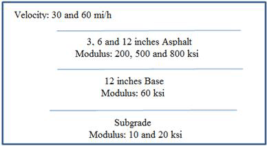
Figure 181 shows a generic pavement structure used in the analyses. For the AC layer, three thickness (3, 6, and 12 inches (76.2, 152.4, 304.8 mm)) and three moduli (200, 500, and 800 ksi (1.37, 3.44, and 5.51 GPa)) were considered. The base layer thickness and modulus were fixed at 12 inches (304.8 mm) and 60 ksi (0.41 GPa), respectively. Moduli of 10 and 20 ksi (0.07 and 0.14 GPa) were used for the subgrade layer. In addition, vehicle speeds of 30 and 60 mi/h (48.3 and 96.6 km/h) were used in the 3D-Move runs. This resulted in 36 combinations of pavement structures and vehicle speeds, as shown in table 63.

1 mi/h = 1.61 km/h

1 inch = 25.4 mm

1 ksi = 6.89 MPa

Figure 181. Illustration. Pavement structures used with 3D-Move analyses.

Table 63. Pavement considered in 3D-Move analyses and corresponding identification key.

Identification Key	AC Modulus at 30 Hz (ksi)	AC Thickness (inches)	Subgrade Modulus (ksi)	Vehicle Speed (mi/h)
B200-3-10-30	200	3	10	30
B200-3-10-60	200	3	10	60
B200-3-20-30	200	3	20	30
B200-3-20-60	200	3	20	60
B200-6-10-30	200	6	10	30
B200-6-10-60	200	6	10	60
B200-6-20-30	200	6	20	30
B200-6-20-60	200	6	20	60
B200-12-10-30	200	12	10	30
B200-12-10-60	200	12	10	60
B200-12-20-30	200	12	20	30
B200-12-20-60	200	12	20	60
B500-3-10-30	500	3	10	30
B500-3-10-60	500	3	10	60
B500-3-20-30	500	3	20	30
B500-3-20-60	500	3	20	60
B500-6-10-30	500	6	10	30
B500-6-10-60	500	6	10	60
B500-6-20-30	500	6	20	30
B500-6-20-60	500	6	20	60
B500-12-10-30	500	12	10	30
B500-12-10-60	500	12	10	60
B500-12-20-30	500	12	20	30
B500-12-20-60	500	12	20	60
B800-3-10-30	800	3	10	30
B800-3-10-60	800	3	10	60
B800-3-20-30	800	3	20	30
B800-3-20-60	800	3	20	60
B800-6-10-30	800	6	10	30
B800-6-10-60	800	6	10	60
B800-6-20-30	800	6	20	30
B800-6-20-60	800	6	20	60
B800-12-10-30	800	12	10	30
B800-12-10-60	800	12	10	60
B800-12-20-30	800	12	20	30
B800-12-20-60	800	12	20	60

1 ksi = 6.89 MPa

1 inch = 25.4 mm

1 mi/h = 1.61 km/h

The impact of pavement temperature was reflected in the AC modulus; therefore, it was not considered an independent parameter. The AC modulus as a function of frequency (a master curve) needs to be specified as input when the viscoelastic material characteristics are considered in 3D-Move. The procedure to build a master curve from AC mix properties is explained in chapter 7. The AC modulus given in table 63 was considered appropriate for a frequency of 30 Hz when estimating the AC moduli as a function of frequency. Table 64 shows the AC mix properties used to develop the master curve for the effort in question.

Table 64. AC mix properties used with 3D-Move analysis.

Variable	Value
Air Voids (percent)	7
Effective binder content (percent)	11
Void filled with asphalt (percent)	61
Percent retained for 0.75 inch	11.62
Percent retained for 0.375 inch	35.3
Percent retained #4 sieve	52.64
Percent passing #200 sieve	7.28
PG grade	58-28
Binder—regression intercept	11.01
Binder—VTS	-3.701

1 inch = 25.4 mm

3D-Move Results and Sensitivity Analysis

The 75 indices listed in table 44 were reevaluated using the 3D-Move results from the 36 pavement structure and vehicle speed combinations detailed in the previous section. The sensitivity of those indices was investigated with respect to the following parameters: AC thickness and modulus, subgrade modulus, and vehicle speed. A major objective of this analysis was to isolate the parameters that most affect the indices. Once identified, those parameters could be used as a starting point in categorizing the pavements in the next step using JULEA.⁽²⁶⁾

For the purpose of brevity, only selected figures showing notable conclusions are presented in this chapter. Similar figures to those presented in this chapter were developed for other deflection indices, but they are not included in this report, as they do not provide further insights. The data used to generate these figures can be obtained directly from FHWA.

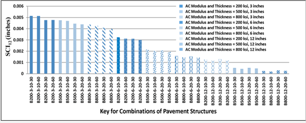
Figure 182 shows the variation of SCI₁₂ for the pavement combinations considered. The x-axis shows the key that can be used to identify easily a specific pavement combination (see table 63). In this graph, nine categories are shown with different fill patterns. For each category, the AC surface layer properties (AC thickness and AC modulus) remained constant. As shown, SCI₁₂, which has been often viewed as an indicator of the influence of the AC layer, is strongly influenced by the AC thickness and modulus.

1 inch = 25.4 mm

Figure 182. Graph. Variation of SCI₁₂ calculated with 3D-Move in simulated pavement combinations.

TS is potentially considered an important index because it is measured directly by the TSD, and thus uncertainties associated with algorithms needed to convert the measured deflection velocities to surface deflections are avoided. In general, TS showed high sensitivity to changes in the pavement layer properties (stiffness and thickness). In particular, TS₄₈ and TS₆₀ seemed to be mostly affected by subgrade modulus. For example, TS₆₀ is clearly influenced by subgrade modulus (see figure 183). As is shown later in this chapter, TS₄ and TS₈ are better correlated with the maximum horizontal strain at the bottom of thin and thick AC layers, respectively.

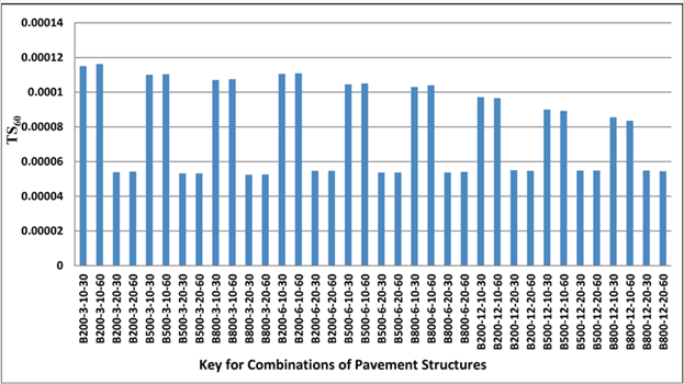
Figure 183. Graph. Variation of TS₆₀ calculated with 3D-Move in simulated pavement combinations.

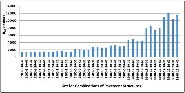
R as defined by Horak was significantly affected by the properties of the surface AC layer and slightly affected by the stiffness of the subgrade.^(62,63) Figure 184 shows the variation in R₆₀ for the pavement combinations considered.

1 inch = 25.4 mm

Figure 184. Graph. Variation of R₆₀ calculated with 3D-Move in simulated pavement combinations.

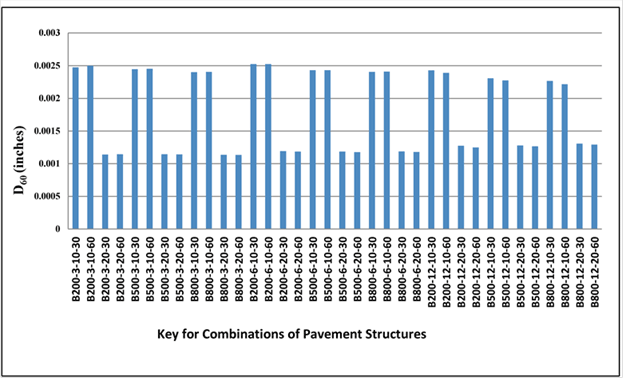
D₆₀ seemed to be the most promising parameter for estimating the subgrade modulus, as shown in figure 185. This parameter seemed to be only affected by the subgrade modulus; other material properties did not have a noticeable influence.

1 inch = 25.4 mm

Figure 185. Graph. Variation of D₆₀ calculated with 3D-Move in simulated pavement combinations.

Figure 186 shows the variation in maximum horizontal strain at the bottom of the AC layer for various pavement combinations considered. Table 65 summarizes the response trends as a few of pavement-related parameters are increased one at a time. As shown in the referenced figure and table, increasing subgrade modulus affected the thin and thick pavements differently. For thin pavements, increasing the subgrade stiffness resulted in an increase in the horizontal strains at the bottom of the AC layer, while the opposite trend was observed for thick pavements (i.e., the strains decreased).

Figure 186. Graph. Variation of maximum horizontal strain at bottom of AC layer in simulated pavement combinations.

Table 65. Effects of an increase in selected pavement parameters on maximum horizontal strain at bottom of AC layer.

Increase in Parameter	Maximum Horizontal Strain at Bottom of AC Layer
AC modulus	Decreased
AC thickness	Decreased
Speed	Decreased
Subgrade modulus	Thin AC (3 inches) increased; thick AC (12 inches) decreased

1 inch = 25.4 mm

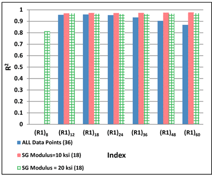
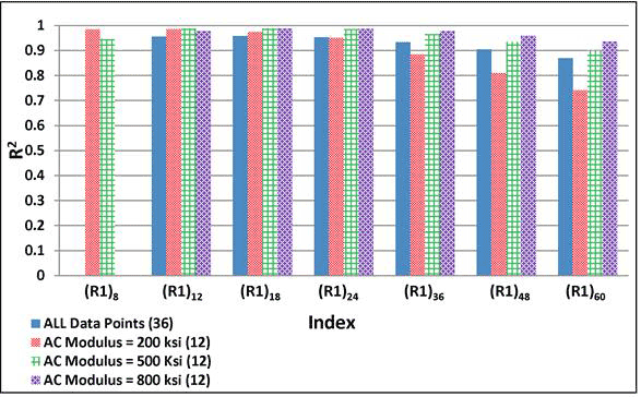
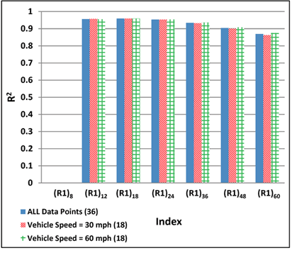
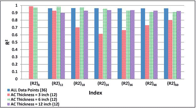
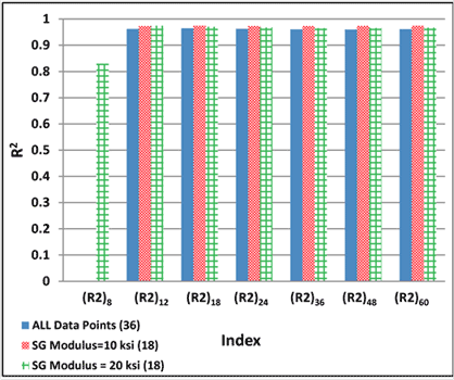
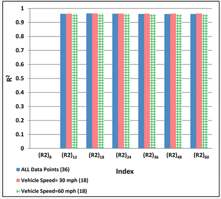
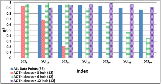
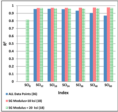
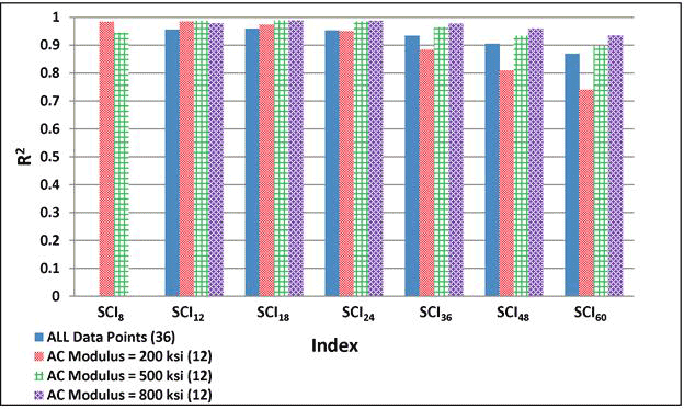
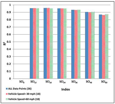
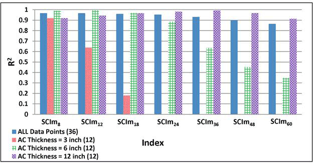
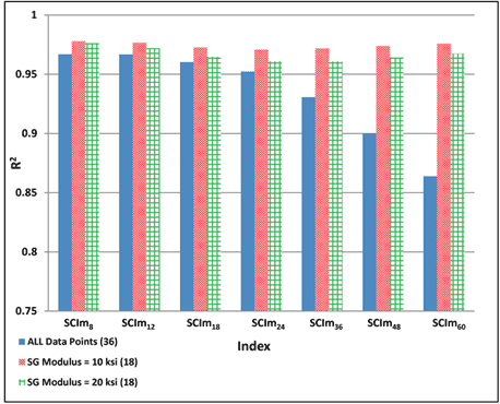
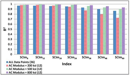
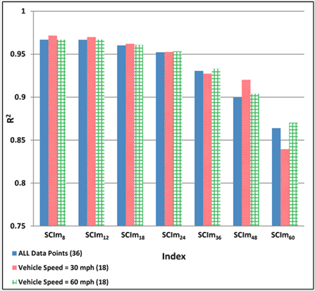
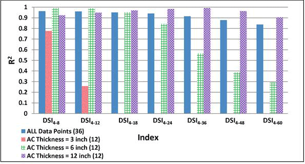
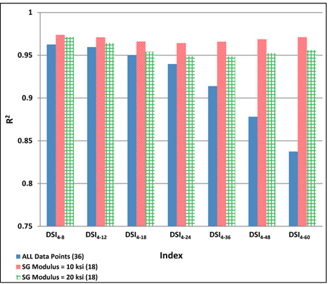
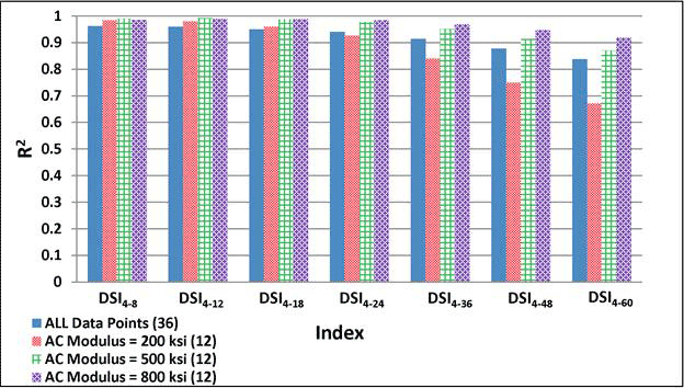
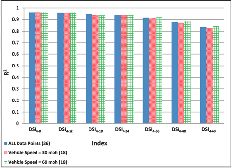
Figure 187 through figure 206 show the variability of the correlations of some of the indices to the maximum horizontal strain at the bottom of the AC layer. In all figures, the numbers within parentheses in the legends indicate the number of data points. One of the important interpretations from these figures is that the AC thickness impacted the strengths of the relationships as judged by the R² values. Many indices did not consistently relate well with the maximum horizontal strain for thin (3 inches (76.2 mm)) AC pavements. Other material properties, such as the subgrade and AC moduli, also influenced the strengths of the relationships for thin pavements. Conversely, thick (12 inches (304.8 mm)) AC pavements were less sensitive to those parameters.

1 inch = 25.4 mm

Figure 187. Graph. Variability of relationships of R1 with maximum horizontal strain at bottom of AC layer for various AC thicknesses.

1 ksi = 6.89 MPa

Figure 188. Graph. Variability of relationships of R1 with maximum horizontal strain at bottom of AC layer for various subgrade moduli.

1 ksi = 6.89 MPa

Figure 189. Graph. Variability of relationships of R1 with maximum horizontal strain at bottom of AC layer for various AC moduli.

1 mi/h = 1.61 km/h

Figure 190. Graph. Variability of relationships of R1 with maximum horizontal strain at bottom of AC layer for various vehicle speeds.

1 inch = 25.4 mm

Figure 191. Graph. Variability of relationships of R2 with maximum horizontal strain at bottom of AC layer for various AC thicknesses.

1 ksi = 6.89 MPa

Figure 192. Graph. Variability of relationships of R2 with maximum horizontal strain at bottom of AC layer for various subgrade moduli.

1 ksi = 6.89 MPa

Figure 193. Graph. Variability of relationships of R2 with maximum horizontal strain at bottom of AC layer for various AC moduli.

1 mi/h = 1.61 km/h

Figure 194. Graph. Variability of relationships of R2 with maximum horizontal strain at bottom of AC layer for various vehicle speeds.

1 inch = 25.4 mm

Figure 195. Graph. Variability of relationships of SCI with maximum horizontal strain at bottom of AC layer for various AC thicknesses.

1 ksi = 6.89 MPa

Figure 196. Graph. Variability of relationships of SCI with maximum horizontal strain at bottom of AC layer for various subgrade moduli.

1 ksi = 6.89 MPa

Figure 197. Graph. Variability of relationships of SCI with maximum horizontal strain at bottom of AC layer for various AC moduli.

1 mi/h = 1.61 km/h

Figure 198. Graph. Variability of relationships of SCI with maximum horizontal strain at bottom of AC layer for various vehicle speeds.

1 inch = 25.4 mm

Figure 199. Graph. Variability of relationships of SCIm with maximum horizontal strain at bottom of AC layer for various AC thicknesses.

1 ksi = 6.89 MPa

Figure 200. Graph. Variability of relationships of SCIm with maximum horizontal strain at bottom of AC layer for various subgrade moduli.

1 ksi = 6.89 MPa

Figure 201. Graph. Variability of relationships of SCIm with maximum horizontal strain at bottom of AC layer for various AC moduli.

1 mi/h = 1.61 km/h

Figure 202. Graph. Variability of relationships of SCIm with maximum horizontal strain at bottom of AC layer for various vehicle speeds.

1 inch = 25.4 mm

Figure 203. Graph. Variability of relationships of DSI_{4 - r} with maximum horizontal strain at bottom of AC layer for various AC thicknesses.

1 ksi = 6.89 MPa

Figure 204. Graph. Variability of relationships of DSI_{4 - r} with maximum horizontal strain at bottom of AC layer for various subgrade moduli.

1 ksi = 6.89 MPa

Figure 205. Graph. Variability of relationships of DSI_{4 - r} with maximum horizontal strain at bottom of AC layer for various AC moduli.

1 mi/h = 1.61 km/h

Figure 206. Graph. Variability of relationships of DSI_{4 - r} with maximum horizontal strain at bottom of AC layer for various vehicle speeds.

Table 66 summarizes the goodness of fit for the relationships between each of the indices considered with the maximum horizontal strain at the bottom of the AC layer using a number of subsets. The subsets considered were AC thickness, subgrade modulus, AC modulus, and vehicle speed. Again, AC thickness was the most influential parameter. Subgrade modulus, AC modulus, and loading speed seemed to affect the most appropriate indices only marginally. However, further classifying the pavements based on subgrade modulus could improve the R² of thin pavements.

Table 66. Variability of the relationships of the indices with maximum horizontal strain at bottom of AC with respect to AC thickness, subgrade modulus, AC modulus, and vehicle speed.

Relationship with Maximum Horizontal Strain	Index	R2 (All Data) (36 Cases)	Sensitivity Analysis with Respect to AC Thickness			Sensitivity Analysis with Respect to Subgrade Modulus		Sensitivity Analysis with Respect to AC Modulus			Sensitivity Analysis with Respect to Vehicle Speed
			3 inches (12 Cases)	6 inches (12 Cases)	12 inches (12 Cases)	10 ksi (18 Cases)	20 ksi (18 Cases)	200 ksi (12 Cases)	500 ksi (12 Cases)	800 ksi (12 Cases)	30 mi/h (18 Cases)	60 mi/h (18 Cases)
R1	R18	N/A	0.9384	0.9777	N/A	N/A	0.8131	0.9841	0.9453	N/A	N/A	N/A
	R112	0.9556	0.6898	0.9931	0.9052	0.9686	0.9681	0.9853	0.9878	0.9784	0.9569	0.9548
	R118	0.9584	0.2165	0.9757	0.9547	0.971	0.9642	0.9741	0.9896	0.988	0.9586	0.9586
	R124	0.9528	Poor	0.9001	0.9775	0.9704	0.9612	0.9507	0.985	0.9871	0.9525	0.9535
	R136	0.9334	Poor	0.6526	0.993	0.9719	0.962	0.8842	0.9654	0.9772	0.9316	0.9354
	R148	0.904	Poor	0.4656	0.9692	0.9741	0.9653	0.8099	0.9343	0.9591	0.8999	0.9079
	R160	0.8691	Poor	0.3587	0.9139	0.9761	0.9684	0.7411	0.8974	0.9348	0.8628	0.875
R2	R28	N/A	0.989	0.9724	N/A	N/A	0.8301	0.9846	0.9492	N/A	N/A	N/A
	R212	0.9614	0.9287	0.9815	0.8977	0.9731	0.9741	0.9898	0.9874	0.9795	0.9628	0.9603
	R218	0.9641	0.7018	0.9741	0.9299	0.9742	0.9703	0.9912	0.9903	0.9876	0.9651	0.9634
	R224	0.9622	0.6138	0.9581	0.9361	0.9729	0.9672	0.9898	0.9896	0.9881	0.9633	0.9614
	R236	0.9602	0.6642	0.9268	0.9348	0.9725	0.9651	0.9866	0.9877	0.9863	0.9622	0.9587
	R248	0.9599	0.7308	0.9103	0.9288	0.9732	0.9654	0.9844	0.9867	0.9848	0.9626	0.9578
	R260	0.9606	0.7989	0.9108	0.9229	0.974	0.9667	0.9834	0.9863	0.9842	0.9638	0.9581
SCI	SCI8	N/A	0.9384	0.9777	N/A	N/A	0.8131	0.9841	0.9453	N/A	N/A	N/A
	SCI12	0.9556	0.6898	0.9931	0.9052	0.9686	0.9681	0.9853	0.9878	0.9784	0.9569	0.9548
	SCI18	0.9584	0.2165	0.9757	0.9547	0.971	0.9642	0.9741	0.9896	0.988	0.9586	0.9523
	SCI24	0.9528	Poor	0.9001	0.9775	0.9704	0.9612	0.9507	0.985	0.9871	0.9525	0.951
	SCI36	0.9334	Poor	0.6526	0.993	0.9719	0.962	0.8842	0.9654	0.9772	0.9316	0.9354
	SCI48	0.904	Poor	0.4656	0.9692	0.9741	0.9653	0.8099	0.9343	0.9591	0.8999	0.9079
	SCI60	0.8691	Poor	0.3587	0.9139	0.9761	0.9684	0.7411	0.8974	0.9348	0.8628	0.875
	SCIm8	0.9668	0.9187	0.9904	0.9179	0.9778	0.9763	0.9804	0.9875	0.9845	0.9715	0.9669
	SCIm12	0.9667	0.6377	0.994	0.9447	0.9766	0.972	0.9832	0.9921	0.9903	0.9699	0.967
	SCIm18	0.9602	0.1804	0.9692	0.9666	0.9726	0.9647	0.9706	0.9908	0.9913	0.9621	0.9608
	SCIm24	0.9522	Poor	0.8868	0.9825	0.9708	0.9608	0.945	0.9846	0.9882	0.9526	0.9533
	SCIm36	0.9305	Poor	0.6355	0.9929	0.9717	0.9609	0.8746	0.9631	0.9762	0.9273	0.9329
	SCIm48	0.8997	Poor	0.4518	0.9677	0.9738	0.9642	0.7975	0.9305	0.9568	0.9201	0.9041
	SCIm60	0.8639	Poor	0.3479	0.913	0.9758	0.9673	0.727	0.8926	0.9317	0.8395	0.8703
DSI	DSI4 - 8	0.9625	0.7765	0.9933	0.9238	0.9737	0.9713	0.9836	0.9898	0.9852	0.9622	0.9629
	DSI4 - 12	0.9595	0.2574	0.991	0.9484	0.971	0.9642	0.9806	0.9918	0.9898	0.959	0.9604
	DSI4 - 18	0.95	Poor	0.9518	0.969	0.966	0.954	0.9594	0.9872	0.9891	0.9417	0.9382
	DSI4 - 24	0.9397	Poor	0.8447	0.984	0.9641	0.9488	0.9256	0.9781	0.9843	0.938	0.9417
	DSI4 - 36	0.9138	Poor	0.5643	0.992	0.9658	0.9486	0.8397	0.9514	0.9694	0.9102	0.9174
	DSI4 - 48	0.8781	Poor	0.3864	0.9632	0.9687	0.9524	0.7501	0.9134	0.9471	0.8719	0.884
	DSI4 - 60	0.8374	Poor	0.2929	0.9046	0.9711	0.9561	0.6711	0.8702	0.919	0.8285	0.8457
	DSI8 - 12	0.9446	Poor	0.9717	0.9629	0.9605	0.9463	0.9614	0.9876	0.9893	0.9432	0.9464
	DSI8 - 18	0.9256	Poor	0.871	0.9788	0.9522	0.9285	0.9163	0.9731	0.9823	0.9256	0.9285
	DSI8 - 24	0.9075	Poor	0.6725	0.9897	0.9502	0.9199	0.86	0.9543	0.971	0.9036	0.9117
	DSI8 - 36	0.8655	Poor	0.3484	0.9848	0.9535	0.9186	0.7354	0.9091	0.9441	0.8584	0.8724
	DSI8 - 48	0.812	Poor	0.2171	0.9358	0.9577	0.923	0.6203	0.8512	0.9092	0.6676	0.8222
	DSI8 - 60	0.7544	Poor	Poor	0.8565	0.961	0.9275	0.5277	0.7894	0.868	0.7399	0.7677
	DSI12 - 18	0.8922	Poor	0.6672	0.9866	0.9387	0.8974	0.8412	0.9432	0.966	0.8872	0.8974
	DSI12 - 24 (BDI)	0.8628	Poor	0.3825	0.9919	0.938	0.8861	0.7578	0.909	0.9438	0.8552	0.8703
	DSI12 - 36	0.7951	Poor	0.147	0.9644	0.9439	0.8845	0.5987	0.8343	0.8961	0.7826	0.8068
	DSI12 - 48	0.7153	Poor	Poor	0.8829	0.9495	0.8896	0.4716	0.7465	0.8392	0.6979	0.5487
	DSI12 - 60	0.636	Poor	Poor	0.7749	0.9534	0.8945	0.3786	0.6604	0.7762	0.6153	0.5881
	DSI18 - 24	0.7944	Poor	Poor	0.9822	0.9324	0.8543	0.6157	0.8302	0.8887	0.7805	0.788
	DSI18 - 36	0.6846	Poor	Poor	0.9042	0.9409	0.8542	0.4414	0.7098	0.8048	0.6483	0.6895
	DSI18 - 48	0.57	Poor	Poor	0.766	0.9476	0.8603	0.3214	0.5832	0.7103	0.5463	0.5796
	DSI18 - 60	0.4695	Poor	Poor	0.6235	0.9519	0.8651	0.241	0.4749	0.6146	0.4447	0.4808
	DSI24 - 36 (BCI)	0.5723	Poor	Poor	0.7995	0.9448	0.8455	0.3289	0.5857	0.7055	0.2316	0.5947
	DSI24 - 48	0.4356	Poor	Poor	0.6131	0.9516	0.853	0.2232	0.4353	0.5747	0.4115	0.4587
	DSI24 - 60	0.3295	Poor	Poor	0.461	0.9558	0.857	0.1565	0.3238	0.4559	0.2184	0.3512
TS	TS4	0.8724	0.9471	0.9807	0.6903	0.8938	0.9635	0.9787	0.9774	0.8763	0.9053	0.8624
	TS8	0.9573	0.1228	0.9911	0.9484	0.9692	0.9612	0.9804	0.9918	0.99	0.9564	0.8925
	TS12	0.9236	0.143	0.9096	0.9741	0.9486	0.9236	0.9199	0.9748	0.9836	0.9209	0.9264
	TS18	0.8431	Poor	0.2844	0.991	0.931	0.8665	0.7226	0.8857	0.929	0.8335	0.8782
	TS24	0.7211	Poor	Poor	0.9486	0.9351	0.8423	0.4949	0.7499	0.8275	0.4878	0.7333
	TS36	0.3756	Poor	Poor	0.5418	0.9545	0.8559	0.1879	0.3685	0.5086	0.354	0.3894
	TS48	0.121	Poor	Poor	0.2052	0.9657	0.8309	Poor	0.1103	0.1754	0.1007	0.1268
	TS60	Poor	Poor	Poor	Poor	0.9631	0.2868	Poor	Poor	Poor	Poor	Poor
SD	SD8	N/A	0.9384	0.9777	N/A	N/A	0.8131	0.9841	0.9453	N/A	N/A	0.9323
	SD12	0.9556	0.6898	0.9931	0.9052	0.9686	0.9681	0.9853	0.9878	0.9784	0.9569	0.9548
	SD18	0.9584	0.2165	0.9757	0.9547	0.971	0.9642	0.9741	0.9896	0.988	0.9586	0.9368
	SD24	0.9528	Poor	0.9001	0.9775	0.9704	0.9612	0.9507	0.985	0.9871	0.9525	0.9558
	SD36	0.9334	Poor	0.6526	0.993	0.9719	0.962	0.8842	0.9654	0.9772	0.93	0.9354
	SD48	0.904	Poor	0.4656	0.9692	0.9741	0.9653	0.8099	0.9343	0.9591	0.8999	0.8665
	SD60	0.8691	Poor	0.3587	0.9139	0.9761	0.9684	0.7411	0.8974	0.9348	0.8628	0.875
Shape factors	F1	0.8367	Poor	0.3641	0.5875	0.9689	0.918	0.7359	0.8497	0.8789	0.793	0.7538
	F2	0.6588	Poor	Poor	0.4127	0.9193	0.885	0.4727	0.6782	0.7676	0.6447	0.1206
Area	A	0.8063	Poor	0.3538	0.5841	0.9669	0.8978	0.7148	0.8219	0.8478	0.7462	0.7591
AUPP	Am	0.9588	Poor	0.9075	0.9805	0.9745	0.926	0.9544	0.9879	0.9899	0.9354	0.9081
Midline surface deflection	D0	0.7719	Poor	0.2321	0.7194	0.9797	0.9302	0.5954	0.7963	0.8559	0.7894	0.7605

1 inch = 25.4 mm

1 ksi = 6.89 MPa

N/A = No correlation exists.

A close examination of the correlations for pavements with AC thicknesses of 3 and 6 inches (76.2 and 152.4 mm) reveals that indices R1₈ ,R2₈, SCI₈, SCIm₈, TS₄, and SD₈ were best related with the maximum horizontal strain with insignificant influence from the AC layer thickness or modulus. Overall, R2₁₂ and SCIm₈ appeared to be the most appropriate indices that were only minimally affected by the AC thickness and other factors studied.

It can also be concluded that increases in AC modulus resulted in an improvement in R² for almost all indices. As explained earlier, TS, which is a direct TSD measurement, is an important index. As shown in table 66, TS₄ had the highest correlations for pavements with AC layer thicknesses of 3 and 6 inches (76.2 and 127 mm), and TS₈ was one of the most appropriate indices for thicker (AC of 12 inches (304.8 mm)) pavements.

Based on the results presented so far in this chapter, it was recommended that the pavements be divided into the following three groups for selecting indices that most appropriate correlate with the maximum horizontal strain at the bottom of the AC surface layer:

• AC surface layer less than 3 inches (76.2 mm).
  
  
• AC surface layer between 3 and 6 inches (76.2 and 152.4 mm).
  
  
• AC surface layer greater than 6 inches (152.4 mm).

For pavements with AC surface layer thicknesses greater than 12 inches (304.8 mm), other pavement layer properties (moduli and thicknesses) did not play an important role. Alternatively, for thinner pavements, the most appropriate indices were affected by the subgrade and base moduli.

Most Appropriate Indices for Correlations with Maximum AC Horizontal Strain Using Available Data

In this subsection, the most appropriate indices using all available runs (43 from step 1 and 36 from step 2, as defined in section 8.1) were explored. The pavement sections for the MnROAD accuracy cells represented pavements that were relatively thin with AC thicknesses varying between 3 and 5 inches (76.2 and 127 mm). Conversely, the pavement combinations considered in step 2 included pavements with AC thicknesses between 6 and 12 inches (152.4 and 304.8 mm). Table 67 shows the reasonable indices (R² > 0.9) when using the combined (steps 1 and 2) database. The total number of reasonable indices with the total database (79 cases) is greater than the number of reasonable indices in step 1 (MnROAD accuracy cells).

Table 67. Most appropriate correlated indices with maximum horizontal AC strain with total database (79 cases).

Best Indices (with Respect to Maximum Horizontal Strain)	Index	R2
R1	R112	0.94
	R118	0.97
	R124	0.95
R2	R212	0.92
	R218	0.96
	R224	0.97
	R236	0.94
	R248	0.90
SCI	SCI12	0.94
	SCI18	0.97
	SCI24	0.95
	SCIm8	0.92
	SCIm12	0.96
	SCIm18	0.97
	SCIm24	0.94
DSI	DSI4 - 8	0.94
	DSI4 - 12	0.97
	DSI4 - 18	0.95
	DSI4 - 24	0.92
	DSI8 - 12	0.96
	DSI8 - 18	0.91
TS	TS8	0.97
SD	SD12	0.94
	SD18	0.97
	SD24	0.95
AUPP	Am	0.95

Summary and Conclusions from 3D-Move Analyses

There are three datasets of 3D-Move runs: (1) MnROAD accuracy cell field trials (step 1); (2) sensitivity analyses with 36 simulated pavement combinations (step 2); and (3) combined data from steps 1 and 2, giving a total of 79 pavement combinations. Table 68 through table 70 presents the reasonable indices with R² greater than 0.9 from step 1 as well as the 20 indices with the highest R² from step 2 and for the combined database. The number of the reasonable indices (R² > 0.9) from step 2 and from the combined database was greater than the reasonable indices from step 1. However, it is important to note that the step 1 pavements only considered AC thicknesses that varied between 3 and 5 inches (76.2 and 127 mm).

Table 68. Most appropriate indices for MnROAD accuracy runs (43 cases) with respect to maximum horizontal strain at bottom of AC.

Best Indices (with Respect to Maximum Horizontal Strain)	Index	R2
R1	R112	0.95
	R118	0.93
R2	R218	0.95
	R224	0.94
SCI	SCI12	0.95
	SCI18	0.93
	SCIm8	0.91
	SCIm12	0.95
	SCIm18	0.93
DSI	DSI4 - 8	0.93
	DSI4 - 12	0.94
	DSI4 - 18	0.91
	DSI8 - 12	0.92
SD	SD12	0.95
	SD18	0.93
TS	TS8	0.94
AUPP	Am	0.91

Table 69. Most appropriate indices for sensitivity analyses (36 cases) with respect to maximum horizontal strain at bottom of AC.

Best Indices (with Respect to Maximum Horizontal Strain)	Index	R2
R1	R112	0.96
	R118	0.96
	R124	0.95
R2	R212	0.96
	R218	0.96
	R224	0.96
	R236	0.96
	R248	0.96
	R260	0.96
SCI	SCI12	0.96
	SCI18	0.96
	SCIm8	0.97
	SCIm12	0.97
	SCIm18	0.96
DSI	DSI4 - 8	0.96
	DSI4 - 12	0.96
SD	SD12	0.96
	SD18	0.96
TS	TS8	0.96
AUPP	Am	0.96

Table 70. Most appropriate indices for combined MnROAD accuracy and sensitivity analysis data (79 cases) with respect to maximum horizontal strain at bottom of AC.

Best Indices (with Respect to Maximum Horizontal Strain)	Index	R2
R1	R112	0.94
	R118	0.97
	R124	0.95
R2	R218	0.96
	R224	0.97
	R236	0.94
SCI	SCI12	0.94
	SCI18	0.97
	SCI24	0.95
	SCIm12	0.96
	SCIm18	0.97
DSI	DSI4 - 8	0.94
	DSI4 - 12	0.97
	DSI4 - 18	0.95
	DSI8 - 12	0.96
SD	SD12	0.94
	SD18	0.97
	SD24	0.94
TS	TS8	0.97
AUPP	Am	0.95

Based on the results from step 1, the following observations and conclusions were made (see table 44 for definitions of indices):

• The influences of TSDD load characteristics (tire spacing, tire load, and inflation pressure) on the indices were investigated, and it was determined that the proposed indices were not sensitive to load characteristics.
  
  
• The indices that best related to the maximum horizontal strain at the bottom of the AC layer in step 1 (higher R² values) are R1₁₂, R2₁₈, SCI₁₂, or SD₁₂. All these indices are based on deflections close to the center of the load.
  
  
• Using D_max instead of D₀ to calculate SCI did not significantly improve the correlation (i.e., similar R² values); however, the use of SCIm did yield slightly better correlations.
  
  
• It appears that using D₄ instead of D₀ to calculate SCI also gave correlations with high R² values. Therefore, if D₄ in TSD measurements is more precise and accurate than D₀, it should be used in the calculation of the indices.
  
  
• Indices based on deflections measured farther away from the load appeared to have better correlations with the vertical subgrade strain. BCI best reflected the role of the lower portion of the pavement system (i.e., the subgrade), and it related better with vertical strains at the top of the subgrade.
  
  
• The most appropriate indices for subgrade vertical strain (R² > 0.95) were as follows:
  
  
  • DSI_{12 - r} = D₁₂ - D_r.
    
    
  • DSI_{18 - r} = D₁₈ - D_r.
    
    
  • DSI_{24 - r} = D₂₄ - D_r.
    
    
• While SCI₁₂ was one of the best correlated indices for horizontal strains at bottom of the AC layers (R² = 0.95), it was not a good index, as indicated by a lower R² value, for subgrade vertical strains (R² = 0.62).

In looking at the combined results from steps 1 and 2, the following observations and conclusions were made:

• D₆₀ seemed to be the most promising parameter to estimate subgrade modulus because it was only affected by the subgrade modulus, while other material properties did not noticeably influence this parameter.
  
  
• TS is the ratio between the vertical particle velocity and the vehicle speed. Since vertical particle velocity is measured directly by TSD, this index is important since no algorithm is required, thus avoiding potential errors in the estimation of D₀ from the direct TSD measurements. TS₄₈ and TS₆₀ were affected only by the subgrade modulus. In general, TS₈ showed high sensitivity to changes in the pavement structural properties. Although TS₈ was overall one of the most appropriate indices from steps 1 and 2 and the combined database, sensitivity analyses showed that TS₄ (for AC thicknesses between 3 and 6 inches (76.2 and 152.5 mm)) and TS₈ (for AC thickness greater than 6 inches (152.4 mm)) provided the best correlations with the maximum horizontal AC strains.
  
  
• The comparison of maximum horizontal AC strains for various pavement combinations revealed the role of the subgrade modulus. Increases in subgrade modulus resulted in increases in horizontal AC strain in thin pavements (AC thickness of 3 inches (76.2 mm)), while the opposite occurred for thicker pavements (AC thickness of 12 inches (304.8 mm)) (i.e., the horizontal AC strains decreased).
  
  
• AC thickness is a critical parameter that should be used to categorize pavements into groups. Subgrade modulus, AC modulus, and loading speed only marginally affected the appropriate indices.
  
  
• An increase in AC modulus increased the R² values for almost all indices.
  
  
• R2₁₂ (Horak's equation) was the overall best index, especially since it was only minimally affected by the AC thickness. SCIm₈ also provided better correlation with maximum horizontal strains for all pavement and speed combinations regardless of AC thickness.

Ultimately, it was recommended that pavements be divided into the following groupings when comparing indices for estimating maximum horizontal strains in the AC surface layer:

• AC surface layer thickness less than 3 inches (76.2 mm).
  
  
• AC surface layer thickness between 3 and 6 inches (76.2 and 152.4 mm).
  
  
• AC surface layer thickness greater than 6 inches (152.4 mm).

For AC thicknesses greater than 12 inches (304.8 mm), other pavement layer properties (e.g., moduli and thicknesses) did not play an important role, while for thinner pavements, the appropriate indices were affected by subgrade and base modulus.

8.4 Step 3: Determining Relationship between Index and Critical Responses from JULEA Analysis

In the previous sections, the 3D-Move analyses identified deflection indices that correlated well with maximum horizontal (or fatigue) strain at the bottom of the asphalt layer. These analyses showed that the correlation between the indices and fatigue strain was most sensitive to the AC thickness; pavements with AC thicknesses less than 3 inches (76.2 mm) were not considered. Also, the analyses identified the best index across the board in situations in which the AC thickness is unknown. Based on these results, the indices summarized in table 71 were considered for further evaluation and development of a deflection index-fatigue strain relationship.

Table 71. Best indices correlating maximum fatigue strain chosen from 3D-Move analyses.

AC Thickness of Pavement Section	Chosen Index from 3D-Move Analysis
Between 3 and 6 inches	R18, R212, R218, SCI8, SCI12, DSI4 - 8, DSI4 - 12, and TS4
Greater than 6 inches	R212, R218, SCI12, SCI18, DSI4 - 8, DSI4 - 12, DSI4 - 18, DSI8 - 12, DSI8 - 18, TS4, TS8, TS12, and AUPP (Am)
Unknown	R212, R218, SCI12, and DSI4 - 12

1 inch = 25.4 mm

As part of the evaluation, a wider range of pavement structures were analyzed using JULEA.⁽²⁶⁾ A database of 15,000 pavement structures was developed using a Monte Carlo simulation, considering a uniform distribution for the modulus and thickness ranges reported in table 72. The corresponding pavement responses (strain and deflections) were computed for each simulated pavement section using JULEA.⁽²⁶⁾ Additionally, a procedure similar to the one used in the 3D-Move analyses (see figure 168) was used to compute the maximum fatigue strain also using JULEA. Similarly, surface deflections at locations detailed in figure 166 were computed. A configuration consisting of 116-psi (799.24-kPa) tire pressure, 13.5-inch (342.9-mm) tire spacing, and 9,000-lb (4,086-kg) load dual tire typically used in TSDDs was used.

Table 72. Pavement property range used in generating database.

Pavement Parameter	Minimum/ Maximum	AC Layer	Base Layer	Subgrade Layer	Stiff Layer
Modulus (psi)	Minimum	100,000	20,000	5,000	2,000,000
	Maximum	1,000,000	80,000	20,000
Thickness (inches)	Minimum	2	4	24	Infinite
	Maximum	16	20	240

1 psi = 6.89 kPa

1 inch = 25.4 mm

Sensitivity Analysis

An effective sensitivity analysis involves a simulation technique that can sample the input variables collectively based on their potential variability and evaluate their effect on a specific distress of a pavement structure. In section 8.3, the computation time involved in 3D-Move analysis limited its utility as a simulation-based sensitivity analysis. Accordingly, the comprehensive JULEA database referenced in the previous section was used to verify the results from 3D-Move sensitivity analyses.⁽²⁶⁾ The JULEA database was first used to identify the most sensitive pavement properties that affected the critical pavement responses. The identified properties were then used to limit the number of 3D-Move sensitivity analysis. The JULEA database was subsequently used to identify the most sensitive deflection indices, which correlated well with fatigue strains.

The Tornado plot was used to visualize the pavement properties (layer stiffness and thickness) that most significantly affected the fatigue strains.⁽⁶⁵⁾ The degree of correlation between fatigue strain and pavement properties was calculated using a rank order correlation coefficient, which is a non-parametric technique for quantifying the relationship between two parameters. The rank order correlation coefficient, r, is independent of the relationship between the input and output. As such, it is well suited for studies that involve analytical models to predict fatigue strain (as is the case here). Rank order correlation uses the position (rank) of a data point in an ordered list to compute its correlation coefficient. The rank order correlation coefficient known as Karl Spearman's r is calculated between the output and each dependent variable as follows:⁽⁶⁵⁾

Figure 207. Equation. Rank order correlation coefficient.

Where:

r = Rank order correlation coefficient.

Δ R = Difference in the ranks between the input and the output values in the same data pair.

n = Number of simulations.

The magnitude of r identifies the extent of correlation between the input and output. The effect of the variable on the predicted response is high when the absolute value of r is close to 1. When r is close to 0, the effect of the variable on the predicted distress is minimal. A positive correlation value indicates that a low value from the input will lead to a low value in the output, and a negative correlation indicates a low value from the input will lead to a high value in the output.

Sensitivity of Pavement Properties on Fatigue Strain

Figure 208 shows the sensitivity of fatigue strain to various pavement properties using the rank-ordered correlation coefficient as determined from the JULEA database of 15,000 pavement structures.⁽²⁶⁾ As shown, AC layer thickness is the most sensitive parameter. Also, the negative correlation for all pavement properties indicates that the increase in each of the simulated pavement properties reduces the maximum fatigue strain. The subgrade stiffness and thickness, for example, had a negligible effect on the maximum fatigue strain.

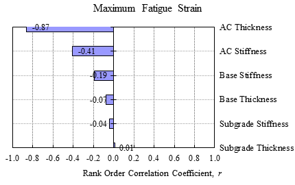
Figure 208. Graph. Sensitivity of pavement properties on maximum fatigue strain.

Sensitivity of Indices to Critical Pavement Design Responses

In section 8.3, it was recommended that pavements be divided into the following AC thickness groupings when comparing indices for estimating fatigue strain:

• AC surface layer thickness less than 3 inches (76.2 mm).
  
  
• AC surface layer thickness between 3 and 6 inches (76.2 and 152.4 mm).
  
  
• AC surface layer thickness greater than 6 inches (152.4 mm).

In this section, the JULEA database of 15,000 pavement structures was grouped based on AC thickness to verify the sensitivity between deflection indices and fatigue strain.⁽²⁶⁾

Pavement Structures with AC Layer Less Than 3 Inches (76.2 mm) Thick

For pavement structures with an AC layer less than 3 inches (76.2 mm) thick, the stiffness of the base, AC, and subgrade layers as well as the thickness of the base layer significantly influenced the fatigue strain. Accordingly, a weak correlation between the deflection indices and fatigue strains was observed only when the AC thickness was considered. Similar trends were observed in the 3D-Move analyses.

It is hypothesized that the contribution of thin AC layers to the measured deflections is limited, and hence other factors must be taken into consideration to establish deflection index-fatigue strain correlations with a high degree of correlation. However, for network-level PMS applications, a relation involving multiple material properties is not practical, and hence such a relation was not pursued further.

Pavement Structures with AC Layer Between 3 and 6 Inches (76.2 and 152.4 mm) Thick

Figure 209 shows the relative sensitivity of maximum fatigue strain to selected deflection indices for pavement structures with an AC layer thickness between 3 and 6 inches (76.2 and 152.4 mm). As shown, all the indices presented in table 71 have relatively good correlation with maximum fatigue strain.

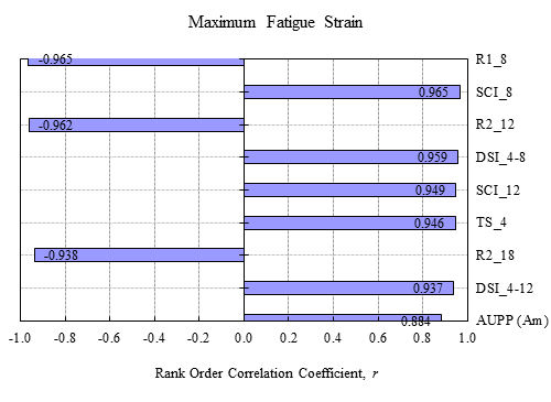
Figure 209. Graph. Sensitivity of curvature index on maximum fatigue strain in thin pavements.

Pavement Structures with AC Layer Between 6 and 16 Inches (152.4 and 406.4 mm) Thick

Figure 210 shows the relative sensitivity of maximum fatigue strain to selected deflection indices for pavement structures with an AC layer thickness between 6 and 16 inches (152.4 and 406.4 mm). As shown, all the indices presented in table 71 had relatively good correlation with maximum fatigue strain.

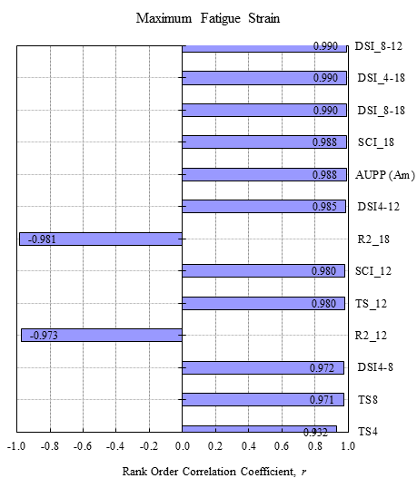
Figure 210. Graph. Sensitivity of curvature index on maximum fatigue strain in thick pavements.

Pavement Structures with Unknown AC Layer Thickness

Figure 209 and figure 210 show that, unlike other indices, the R2₁₂ index appears to be a reasonable predictor of maximum fatigue strain for pavements with both thin and thick AC layers. Accordingly, when the AC thickness is not known, the R2₁₂ index can be used to estimate maximum fatigue strains based on measured TSDD deflections, as suggested by the 3D-Move sensitivity analyses.

Relationship between Indices and Critical Response

Incorporating TSDD measurements into network-level PMS applications requires an established relationship between the computed or measured indices and fatigue strain. In this section, the fatigue strain was related to the indices deemed sensitive in the previous section and also from the 3D-Move analysis. Table 73 presents the relationships developed for pavement structures with thin (3 to 6 inches (76.2 to 152.4 mm)) and thick (6 to 16 inches ((152.4 to 406.4 mm)) AC layers. The correlation coefficient associated with each relationship is also presented in the table. For thin AC layers, separate relationships were developed for those cases where the AC layer thickness (H1) is greater than the base layer thickness (H2) (i.e., H1/H2 > 1).

Table 73. Relationship between curvature indices and maximum fatigue strain.

AC Layer Thickness	Pavement Sections	Chosen Best Indices	Relation	R2
Thin (3 to 6 inches)	All	SCI8 (mil)	98.754 × SCI80.8915	0.93
	(H1/H2) > 1		100.79 × SCI80.8958	0.96
Thick (6 to 16 inches)	All	SCI18 (mil)	40.224 × SCI180.9257	0.98
Unknown	All	R212 (inches)	337974 × R212-0.779	0.97

1 inch = 25.4 mm

Because the relations between the deflection indices and maximum fatigue strain can be sensitive to AC layer thickness, better predictions of the maximum fatigue strains are possible when the AC thickness is known or measured during the TSDD testing. The JULEA database was used to categorize the pavement structures according to AC layer thickness in 1-inch (25.4-mm) intervals.⁽²⁶⁾ Each group contained about 1,000 pavement structures within the pavement properties presented in table 72. Table 74 summarizes the relationships between the most sensitive deflection indices and the fatigue strain for each group. The correlation coefficient for each relationship is also presented in table 74.

Table 74. Relationship between curvature indices and critical pavement responses with known AC thickness.

AC Layer Thickness (inches)	Unbound Layer Properties	Chosen Index	Range of Indices Value (mil)	Maximum Fatigue Strain (microstrain)	R2
3–4	Base 20–80 ksi and 4–12 inches; subgrade 5–20 ksi and 24–240 inches	SCI8	1.59 to 8.55	83.958 x SCI80.9903	0.90
4–5			1.23 to 6.65	90.107 x SCI81.0049	0.95
5–6			0.96 to 4.83	98.847 x SCI80.9723	0.97
6–7	Base 20–80 ksi and 4–20 inches; subgrade 5–20 ksi and 24–240 inches	SCI18	1.87 to 10.22	36.295 x SCI181.0096	0.92
7–8			1.58 to 11.07	37.106 x SCI181.0029	0.95
8–9			1.38 to 7.33	38.252 x SCI180.986	0.97
9–10			1.16 to 7.45	39.638 x SCI180.9611	0.98
10–11			1.02 to 6.89	40.933 x SCI180.9195	0.97
11–12			0.87 to 6.07	41.393 x SCI180.894	0.97
12–13			0.79 to 5.1	41.505 x SCI180.8672	0.96
13–14			0.69 to 4.68	41.301 x SCI180.8283	0.95
14–15			0.63 to 4.23	40.361 x SCI180.8313	0.96
15–16			0.59 to 4.27	39.278 x SCI180.7978	0.95

1 inch = 25.4 mm

ksi = 6.89 MPa

Effect of TSDD Loading Configuration

The RWD and TSD used in the MnROAD field trials had different loading configurations, as summarized in table 75. To study the effect of loading configuration on the relationship between deflection index and fatigue strain, a separate database of 50,000 pavement structures, each subjected to the TSD and RWD loading configurations, was simulated within the pavement properties presented in table 72.

Table 75. Loading configuration of TSDD used in the field test.

TSDD Equipment	Dual Tire Load (lb)	Tire Pressure (psi)	Dual Tire Spacing (inches)
TSD	11,150	116	13.5
RWD	9,500	100	14.5

1 lb = 0.454 kg

1 psi = 6.89 kPa

1 inch = 25.4 mm

Figure 211 and figure 212 show the relationships between SCI₁₂ and fatigue strain for the RWD and TSD loading configurations, respectively. The similarity between the two confirms that the proposed relationships are not dependent on the loading configuration, as was also found during the 3D-Move analysis.

1 mil = 0.0254 mm

Figure 211. Graph. General relationship between maximum fatigue strain and SCI for RWD loading.

1 mil = 0.0254 mm

Figure 212. Graph. General relationship between maximum fatigue strain and SCI for TSD loading.

8.5 Field Evaluation of Indices

So far, the focus of this chapter has been mostly on numerical analyses in order to recommend the most appropriate indices. In this section, the estimated TSD accuracies and precisions reported in chapter 6 were used to estimate the most practical and robust indices among those reported in previous sections. For this evaluation, the TSD new deflection algorithm discussed in chapter 5 was used since the old method did not provide enough data points for the analyses. Since the new TSD algorithm provides deflections at 4-inch (100.6-mm) intervals, including D₀, only indices that conformed to this spacing were addressed. These values, along with the TS directly measured by the TSD, were used to evaluate the precision and accuracy of the most appropriate indices using the data collected during the MnROAD testing. The following subsections describe the process and the results obtained from such evaluation. It should be noted that the trends and recommendations in this section are based on the limited data collected during the MnROAD field testing and are subject to the uncertainties associated with the measurements and analyses enumerated for the accuracy and precision studies outlined in chapters 5 and 6.

Accuracy

For the accuracy evaluation, the selected indices from the TSD were compared with the same indices calculated from the deflection or velocity basins measured with geophone 3 at all cells. The accuracy was evaluated in terms of the percentage of difference as established in chapters 5 and 6 for the deflection slopes irrespective of the AC thickness recommendations for estimating the strains. Figure 213 presents the results from such evaluation. The error bars in the figure correspond to the 25th and 75th percentile ranges of the difference. A 15 percent threshold median difference, which was considered as a reasonable level of difference given the state of the technology, was also added to the plot shown in figure 213. The indices based on the deflection slopes yielded lower difference values as compared to the other indices. The indices based on R seem to be the least accurate.

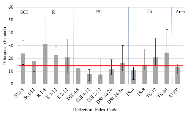
Figure 213. Graph. Accuracy evaluation of indices.

Precision

As presented in section 6.3, the new TSD vertical deflection estimates were found to be less precise than the deflection slope measurements. For this evaluation, precision was incorporated using the same approach but with a slightly different presentation of results. As in chapter 6, the SEE values and ranges were estimated for each index and cell. The median COV, obtained from the ratio between the median SEE and the median range, was used to quantify the precision of each deflection index irrespective of the AC thickness recommendations for estimating the strains. Figure 214 shows the resulting median COVs as well 25th and 75th percentile ranges of the COVs. A 15 percent threshold median COV was also added to the plot as a reasonable precision. Most indices were under this 15 percent threshold COV. As shown, the indices based on the deflection slopes performed better than those based on the TSs by themselves. The three R indices performed the worst, with median COVs ranging from 29 to 40 percent.

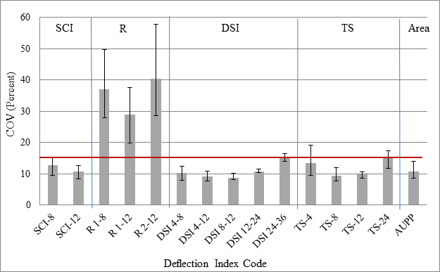
Figure 214. Graph. Precision evaluation of indices.

Overall Field Results

To easily visualize the overall performance of these indices, figure 215 was developed by combining figure 213 and figure 214. This plot, which presents the precision results on the abscissa and the accuracy results on the ordinance, is segmented into four quadrants to further characterize the performance of the indices in question. As shown, the most robust indices are those in the lower left quadrant (marked in green) and include four DSIs, TS₄, and AUPP. The indices in the upper left quadrant (TS and SCI) may also be considered as reasonably precise but not as accurate as those in the lower left quadrant. Based on this study, the three radii of curvature indices under consideration do not seem to yield accurate enough results since they all fall in the upper right-hand quadrant (i.e., quadrant with low accuracy and precision marked in red). DSI_{4 - 12} was found to be the most robust index based on the TSDD accuracy and precision analyses conducted in this study.

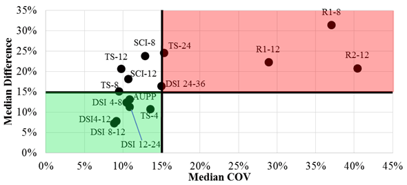
Figure 215. Graph. Overall field performance of indices.

The uncertainties of the modeled indices were evaluated by dividing the SEE in estimating the maximum fatigue strain by the median range of calculated strains for each of the indices for different AC thicknesses as described previously. The results from such analysis are presented in figure 216. This figure depicts the same 15 percent threshold as described in section 8.5. Most of the indices have a median COV below 15 percent except for the ones used to determine the strain for unknown pavement thickness.

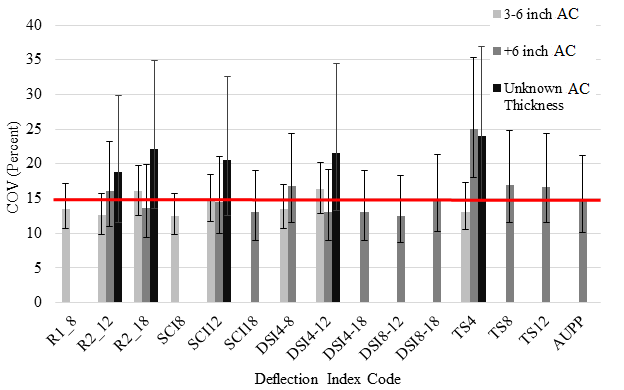
1 inch = 25.4 mm

Figure 216. Graph. Precision of modeled indices in different pavement thicknesses<

8.6 Summary

The overall performance of the selected indices was evaluated by combining the field and JULEA results.⁽²⁶⁾ The outcomes from figure 214 through figure 216 were combined into table 76. Indices were then ranked within their pavement thickness ranges according to a performance number (see table 77). The device precisions, device accuracies, and model uncertainties were assigned values of 1 (poor) when their COV values were greater than 20 percent, 3 (fair) when their values were between 10 and 20 percent, and 5 (good) for values less than 10 percent. Similarly, the R² values were assigned 1 (poor) for values less than 0.90, 3 (fair) for values between 0.90 and 0.95, and 5 (good) for values above 0.95.

Table 76. Summary of performances of different indices.

AC Thickness of Pavement Section	Index	Units	Precision COV (Percent)	Accuracy (Percent Difference)	Model COV (Percent)	Model R2
Between 3 and 6 inches	DSI4 - 12	mil	9	8	16	0.88
	SCI12	mil	11	18	15	0.90
	DSI4 - 8	mil	10	12	13	0.92
	TS4	mil/inch	14	11	13	0.91
	SCI8	mil	13	24	12	0.93
	R18	inches	37	31	14	0.93
	R212	inches	40	21	13	0.93
Greater than 6 inches	DSI4 - 12	mil	9	8	13	0.97
	DSI8 - 12	mil	9	7	12	0.98
	SCI12	mil	11	18	14	0.96
	DSI4 - 8	mil	10	12	17	0.95
	TS8	mil/inch	9	15	17	0.94
	TS12	mil/inch	10	21	17	0.96
	AUPP	mil	11	13	15	0.97
	R212	inches	40	21	16	0.95
	TS4	mil/inch	14	11	25	0.87
Unknown	DSI4 - 12	mil	9	8	22	0.97
	SCI12	mil	11	18	20	0.97
	R212	inches	40	21	19	0.97
	TS4	mil/inch	14	11	24	0.93

1 inch = 25.4 mm

1 mil = 0.0254 mm

1 mil/inch = 0.0001 mm/mm

Table 77. Ranking of different indices.

AC Thickness of Pavement Section	Index	Units	Device Precision	Device Accuracy	Model Uncertainty	Model R2	Overall Performance (1–5)
Between 3 and 6 inches	DSI4 - 12	mil	5	5	3	1	3.5
	SCI12	mil	3	3	3	3	3.0
	DSI4 - 8	mil	3	3	3	3	3.0
	TS4	mil/inch	3	3	3	3	3.0
	SCI8	mil	3	1	3	3	2.5
	R18	inches	1	1	3	3	2.0
	R212	inches	1	1	3	3	2.0
Greater than 6 inches	DSI4 - 12	mil	5	5	3	5	4.5
	DSI8 - 12	mil	5	5	3	5	4.5
	SCI12	mil	3	3	3	5	3.5
	DSI4 - 8	mil	3	3	3	5	3.5
	TS8	mil/inch	5	3	3	3	3.5
	TS12	mil/inch	5	1	3	5	3.5
	AUPP	mil	3	3	3	5	3.5
	R212	inches	1	1	3	5	2.5
	TS4	mil/inch	3	3	1	1	2.0
Unknown	DSI4 - 12	mil	5	5	1	5	4.0
	SCI12	mil	3	3	1	5	3.0
	R212	inches	1	1	3	5	2.5
	TS4	mil/inch	3	3	1	3	2.5

1 inch = 25.4 mm

1 mil = 0.0254 mm

1 mil/inch = 0.0001 mm/mm

Note: A ranking of 1 indicates poor, a ranking of 3 indicates fair, and a ranking of 5 indicates good.

The overall performance was then determined by assigning a 25 percent importance to each of the four parameters (device precision, device accuracy, model uncertainty, and R²) and obtaining a weighted average of the four parameters. Indices that required a deflection parameter of 18 inches (457.2 mm) were not included in this table since TSD did not report a value at that distance. DSI_{4 - 12} appears first on the three different AC thicknesses categories. SCI₁₂ also performed well in the three AC thickness categories with an overall performance of 3 or higher. It should be noted that device accuracy can be improved if the effectiveness of the deflection algorithm is improved. At a minimum, the TSD old deflection algorithm, which was identified in accuracy analysis (section 6.2) to be better than new deflection algorithm, can be modified to compute the deflections at the locations needed to determine the identified effective indices.

In considering the results and conclusions presented in this chapter, it is important to recognize that a limitation of the analyses is that the device precision and accuracy were obtained for pavements with a AC thickness of 5 inches (127 mm) or less if the full depth reclamation with engineered emulsion is not considered as AC. The most robust index, DSI_{4 - 12}, is related to maximum fatigue strain using the JULEA database and is presented in table 78.

Table 78. Relationship between robust TSD index DSI_{4 - 12} and critical pavement responses with unknown and known AC thickness.

AC Layer Thickness (inches)	Maximum Fatigue Strain (microstrain)	R2
3–6 (thin AC)	69.1 x DSI4 - 120.9348	0.88
6–16 (thick AC)	76.22 x DSI4 - 120.8924	0.97
Unknown	76.24 x DSI4 - 120.8969	0.97
3–4	66.96 x DSI4 - 120.9351	0.77
4–5	62.567 x DSI4 - 121.0174	0.88
5–6	64.66 x DSI4 - 121.0379	0.94
6–7	71.646 x DSI4 - 121.0005	0.96
7–8	74.381 x DSI4 - 120.9757	0.97
8–9	76.458 x DSI4 - 120.9427	0.98
9–10	77.802 x DSI4 - 120.9107	0.97
10–11	77.868 x DSI4 - 120.8674	0.96
11–12	76.861 x DSI4 - 120.8395	0.95
12–13	75.154 x DSI4 - 120.8149	0.95
13–14	72.194 x DSI4 - 120.778	0.94
14–15	70.196 x DSI4 - 120.7824	0.94
15–16	66.402 x DSI4 - 120.7525	0.93

1 inch = 25.4 mm

8.7 Temperature Correction Procedure

The deflection parameter measured by the TSDD is a function of pavement temperature at the structural evaluation. Consistent evaluation and tracking of the index computed from deflection parameters over the pavement service period requires the maximum fatigue strains computed from the index to be corrected to a standard reference temperature. The recommended approach, developed as part of the project, is as follows:

1. Compute temperature correction factor, T_c, as follows:
   
   




Figure 217. Equation. Temperature correction factor.

* Modified November 21, 2016

Where:

T_f (°F) = Temperature at time of the TSDD field measurements.

T_r (°F) = Reference temperature, which should be set to 70 °F (21.11°C).

2. Compute dynamic modulus (E_f) based on computed strains and AC layer thickness using relations presented in table 79.
   
   
3. Compute dynamic modulus at reference temperature, E_r of 70 °F (21.11°C) as follows:
   
   



Figure 218. Equation. Dynamic modulus at reference temperature.

4. Compute temperature corrected strains using the computed dynamic modulus at reference temperature (E_r) and the inverse of the relations presented in table 79.

While the correlation coefficients for the relations in table 79 are not high, the error in the temperature corrections is expected to be minimal because the same relations are used to compute the AC dynamic modulus from the computed strains and then to re-compute the strains from the temperature corrected AC dynamic modulus.

Table 79. Relationship between maximum fatigue strain (ε) and AC modulus for temperature correction.

AC Layer Thickness (inches)	Relation Between Maximum Fatigue Strain and AC Modulus	R2
3–4	5.28E+08 x ε max-1.27	0.47
4–5	6.56E+08 x ε max -1.36	0.59
5–6	7.23E+08 x ε max-1.44	0.62
6–7	6.39E+08 x ε max-1.46	0.67
7–8	4.96E+08 x ε max-1.46	0.68
8–9	4.91E+08 x ε max-1.51	0.72
9–10	3.68E+08 x ε max-1.49	0.76
10–11	3.29E+08 x ε max-1.51	0.77
11–12	2.88E+08 x ε max-1.52	0.79
12–13	2.50E+08 x ε max-1.53	0.83
13–14	2.30E+08 x ε max-1.55	0.83
14–15	1.61E+08 x ε max-1.49	0.85
15–16	1.45E+08 x ε max-1.51	0.85