MEPDG Traffic Loading Defaults Derived From Traffic Pooled Fund Study

CHAPTER 5-METHODOLOGY FOR ESTIMATING RELIABILITY OF TRAFFIC LOADING DATA

RESEARCH OBJECTIVE

One of the objectives of this study was to develop a procedure for estimating the reliability of the traffic load data used for pavement design. In this study, traffic loading data reliability was estimated in terms of the maximum expected error in percentages of axles in NALS used for pavement design for a given CL.

Based on the reliability approach used in the MEPDG, there is no direct relationship between the reliability of MEPDG outcomes and the accuracy of the specific inputs. The measurement error of all inputs is included indirectly through the standard error of each transfer function. The standard errors used to define reliability in the MEPDG are distress-specific and were derived from the calibration of the transfer functions. The standard error represents the total model error. It is difficult to consider or evaluate the effect of an individual measurement error (measurement of axle load) on performance predictions. Specifically, there is no means within the MEPDG to directly consider traffic load data reliability as a direct pavement design input. However, knowledge of traffic loading data reliability is useful in developing data selection criteria for generating accurate traffic loading inputs for the MEPDG.

In this study, the research team developed a traffic loading data reliability procedure to facilitate the evaluation of WIM data accuracy and to aid in the development of data selection criteria for generating MEPDG traffic loading inputs and defaults. In other words, the procedure addresses the issue of quantifying and/or reducing the variability of WIM data for making a decision on the input to the MEPDG.

SOURCES OF ERROR AND VARIABILITY IN TRAFFIC LOADING DATA

Sources of Error

To develop NALS for pavement design, it is necessary to estimate the percentage of loads for each axle group type within each load range (load bin) of the load spectrum. In the case of global traffic loading defaults, such percentages typically represent normalized load distribution for a typical day of the year. In the case of site-specific traffic loading inputs, such percentages should represent the load distribution for a typical day of each calendar month. These NALS estimates are computed using the number of axle counts within each load range collected over a certain period of WIM monitoring.

The number of axle counts per load range (bin) can be represented using the following equation:

Figure 11. Equation. Number of axle counts per load range (bin).

Where:

N_ij = WIM-measured number of counts within load range i for axle group type j.

Nact_ij = Actual number of counts within load range i for axle group type j.

ε_ijk = Error associated with factor, k, for load range i for axle group type j.

Some typical factors (k) causing errors in load counts include the following:

• Equipment-related factors:
  
  
  • Accuracy of axle load measurements (WIM precision and bias).
    
    
  • Equipment malfunction or improper calibration.
    
    
• Data interpretation or the incorrect placement of measured values in the correct bins (i.e., inaccurate axle group type or vehicle class assignment).
  
  
• Small sample size (number of monitoring days and their distribution over time).
  
  
• Procedure to estimate the percentages of axle loads.

Each of these factors has a different importance for the NALS estimation process. Some may have significant impacts on the estimates, and criteria for gathering and using data must be established to mitigate these impacts.

In addition to errors associated with the NALS estimate, there is another important source of uncertainty related to traffic inputs for pavement design that may be even more important: the estimate of truck traffic volume and weights over time. For pavement design, it is necessary to estimate future truck traffic volume. Such estimates are subject to large variations that have major impacts on pavement performance; however, it was not within the scope of this study to evaluate these errors. This study addresses only factors affecting the reliability of axle loading data collected using WIM systems.

Error Versus Variability

It is important to understand the difference between error and variability when addressing the various sources of error. When measuring an axle load using a WIM system, a certain error may be expected, and its magnitude is associated with the accuracy of the WIM system in place. For example, for a WIM system that has accuracy in axle weight measurement within 20 percent of the true or actual value with 95 percent confidence, for an axle load of 10,000 lb, the error will be less than 2,000 lb in approximately 95 percent of all the measurements, assuming the equipment has no bias. Therefore, when counting the number of loads between 9,000 and 11,000 lb, the count may be different from the true number of counts due to axle weight measurement error associated with WIM accuracy.

However, when making WIM measurements over a given period, the number of counts within the load range may also be different because of the daily and seasonal variations in traffic. The differences in counts due to such variations cannot be attributed to measurement error but to inherent variations in traffic for that specific WIM site location. This relates to having insufficient data to provide an accurate representation of the actual NALS for that site. Variation in traffic volume, coupled with limited data availability, may result in errors in DOW, monthly, or annual traffic loading estimates.

For example, if the percentage of loads within a specific range is estimated for the month of May, but WIM measurements were taken for only 2 days in May, a difference in estimates will be found if all 31 days in May are used. Moreover, if the 2 days of measurement were taken during the weekend, a larger difference could be expected due to the potential larger variations in traffic volume or loading distribution between weekdays and weekends. Similar errors may be introduced if the number of weekdays and weekend days in the month are not properly weighted when the full month of data is unavailable. In addition, an annual spectrum represents the distribution of traffic loads during a full year, so errors from data gaps in months or partial months may also impact the final estimated load spectra. Such errors can be mitigated by increasing the sample size.

SCOPE OF SUPPORTING ANALYSES

The research team conducted a number of statistical analyses to identify and evaluate the impact of different sources of errors in axle load measurements on the calculation of NALS. The methodology for statistical analyses was as follows:

1. Define a parameter for assessing accuracy and reliability of axle load spectrum.
   
   
2. Identify different sources of errors affecting accuracy of axle load spectrum and review SPS TPF WIM precision and bias requirements.
   
   
3. Conduct statistical tests to aid in evaluation of errors associated with WIM equipment measurements, data availability, and data variability, and determine relative significance of different sources of error.
   
   
4. Use findings from data analyses to develop traffic loading data selection criteria, considering reliability of traffic load data for pavement design.

The following sections describe each step in greater detail.

STATISTICAL PARAMETER FOR ASSESSING AXLE LOAD SPECTRUM RELIABILITY-PWLE

Purpose

A major component of the proposed procedure for estimating the reliability of the traffic load data is the development of a parameter that can be used to represent the reliability of the whole axle load spectrum for pavement design. This parameter can be viewed as a representative error for load ranges of the axle load spectrum, and its magnitude is a function of the selected CL.

Definition

For this study, the research team developed a new parameter: the PWLE for the spectrum. PWLE is a single value that provides a representative estimate of expected errors in percentages of axle load counts for individual load bins in NALS for a selected CL. PWLE is designed to aid in traffic loading data selection for MEPDG design and analysis, as it takes into consideration both the relative percentage of the traffic at each load level and the impact of each load level on the MEPDG-based pavement performance predictions.

PWLE accounts for some major pavement performance and statistical factors in one parameter, including the following:

• The variability of estimated axle frequency for each load bin of the spectrum.
  
  
• The importance of each individual load bin relative to other bins in the load spectrum, represented by the frequency of axle counts (or percentage of axle loads) within the specific load range (load bin).
  
  
• The importance of the load level associated with each load bin on pavement performance, represented by the weight factor associated with each load bin and developed in this study using MEPDG runs. The approach was presented in chapter 4.

PWLE can be viewed as a representative value rather than a statistical estimate of a single probability distribution. Although some load bins in NALS may have larger or smaller errors, PWLE is representative of the whole spectrum and reflects more weight for errors associated with load bins that have higher percentage of counts, as well as those that comprise higher load magnitudes (load bins that contain heavy loads, counts, or percentages) that have a greater impact on pavement performance.

PWLE Formulation

With PWLE, an error representing the entire NALS is determined based on a selected CL. The general PWLE formula is presented in figure 12.

Figure 12. Equation. PWLE for the selected CL.

Where:

PWLE = For the selected CL; it represents the error associated with an estimate of NALS.

CF = Confidence factor; depends on the desired CL for the error assuming the error is normally distributed (see table 5). CF is a function of the sample size n and CL.

n = Sample size; may represent the number of days used to estimate the monthly spectrum or the number of months used to estimate the annual spectrum for an individual site.

i = Load bin number in the load spectrum.

nb = Total number of load bins in axle load spectrum for axle group type j (e.g., for single axle spectrum, nb = 39).

j = Axle group type (j = 1 for single, 2 for tandem, 3 for tridem, and 4 for quad).

nt = Number of axle group types considered in the calculation of PWLE; nt is 4 when all axle group types (single, tandem, tridem, and quad) are considered, or it can be 1 if only one axle group type is considered.

vⁿ_ij= Variance of the axle count percentages for load bin i and axle group type j over n days or months and is calculated from the data (P_ijk) used to estimate.

W_ij = Weight factor (based on the importance of the load level for pavement design) for axle group type j and the load level (load bin) i (see table 4). This parameter depends only on the axle group type j and the load bin i.

= Average percentage of axle loads for load range i and axle group type j for the number of days or number of month n considered. When PWLE is estimated for an annual NALS computed for an individual site, n is the number of months used in the NALS calculation, and P_ijk values represent the percentage of axle loads for load range i and axle group type j for month k. When PWLE is estimated for a monthly NALS computed for an individual site, n is the number of days and P_ijk values represent percentage of axle loads for load range i and axle group type j for day k.

p_j = Percentage of total axle counts that belong to axle group type j based on the total number of days or months, depending on the purpose of PWLE computation.

*Based on Microsoft Excel^® TINV compatibility function.

PWLE may also be used to estimate the pooled error for a specific vehicle class or even for a specific axle group type. The general formula is valid for both cases, and examples of these calculations are presented later in this report.

Parameters Considered in PWLE Computation

The rationale for the PWLE parameter is that it considers the expected errors and deviations for each load range of the spectrum and pools the associated variances according to the expected percentage of traffic for the specific load range and axle group type. In addition to load frequency, it considers a performance weight, W_ij, that is associated with the relative impact that the specific load range and axle group type has on pavement performance. Using this approach, both the impact of the load level for each axle group type and relative percentage of traffic in each load range are taken into consideration to estimate the representative error of the spectrum.

Figure 13 presents the approach for considering both frequency and importance of axle loads at different load levels in PWLE estimation. Each axle group type j and load bin i has a corresponding performance weight factor W_ij and percentage of loads P_ij. The higher the load, the higher is the performance weight factor. The relationship between load level and W_ij is based on pavement performance estimated using the MEPDG (see chapter 4).⁽⁴⁾

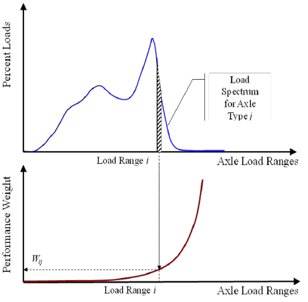
Figure 13. Graph. Estimation of parameters for PWLE.

Parameters P_ijk and

P_ijk is the percentage of axle loads in NALS for load bin i, axle group type j, and time period (day or month) for which NALS is computed. When multiple NALS are used to estimate an average NALS (such as monthly NALS used to estimate annual NALS), the average percentage of axle loadsis calculated for each load bin i, axle group type j, and month k.

Computation of P_ikj and is dependent on how PWLE is used as follows:

• PWLE to characterize errors associated with monthly NALS for a given site:
  
  
  • P_ijk is the percentage of axle loads for load range i and axle group type j and day k in daily NALS for a given site.
    
    
  • is the average daily percentage of axle loads for load range i and axle group type j calculated for the month using data for n available days in the month. In this case,represents the average daily percentage of axle loads for load range i and axle group type j for a typical day of the given month.
    
    
• PWLE to characterize errors associated with annual NALS for a given site:
  
  
  • P_ijk is the percentage of axle loads for load range i and axle group type j and month k in monthly NALS for a given site_.
    
    
  • values computed for individual months are averaged to obtain avalue. In this case,represents the annual average percentage of axle loads for load range i and axle group type j. NALS for 12 calendar months (n = 12) are recommended to compute the annualvalue.

Parameter n

Depending on the purpose of the PWLE, n represents the number of days. It may also represent month, number of months, or year.

Parameter v_ij

Variance v_ij is obtained by calculating the square of the differences of the P_ijk deviations from the averagefor each load bin. These deviations are computed for each day, each month, or each site depending on what PWLE represents. Based on the PWLE application, v_ij is obtained either for each month (if PWLE is based on daily traffic data for a month) or for each year (if PWLE is based on monthly traffic data for at least 1 year.)

For example, if PWLE is calculated for the year, the variance is calculated from the standard deviation of P_ij (for each load bin i and axle group type j) between the 12 months representing the annual traffic. Monthly NALS estimates that are used in computation of the variances for PWLE incorporate all sources of error as well as daily traffic data variation. Therefore, by using the monthly variances, the overall error associated with WIM data is being assessed.

Parameter p_j

The p_j parameter is used in PWLE to quantify the percentage of axle counts that belong to axle group type j in relation to total axle counts.

PWLE Applicability

PWLE was developed for this study to aid in evaluating traffic load data reliability in terms of the expected error in percentages of axles in the NALS for a given CL. This could be done for an overall axle load spectrum developed for a given site (considering all vehicle classes and axle group types) or for an individual vehicle class and axle group type.

PWLE can be used to evaluate different WIM data availability scenarios and equipment performance characteristics. The parameter allows the user to evaluate the expected error associated with the axle load spectrum that is reflective both of the relative percentage of the axle loads in each load bin and its potential impact on pavement performance based on MEPDG load-associated distress models or load equivalency factors. PWLE could be used to evaluate the following:

• Reliability of load spectrum as a function of the number of monitoring days in a given month or the number of months of available data for a given site.
  
  
• Effect of different WIM performance characteristics (precision and bias) on reliability of NALS estimates.
  
  
• Effect of different WIM site conditions and WIM technology used on reliability of NALS estimates.
  
  
• Differences in variability/reliability of NALS estimate using data before and after WIM system calibration.

Knowledge gained though these analyses could be applied to define WIM data selection criteria for the development of unbiased and reliable NALS estimates.

PROCEDURES FOR ESTIMATING RELIABILITY OF TRAFFIC LOADING DATA

Approach

During this study, the researchers developed several procedures for assessing the reliability of NALS estimates to evaluate the impact of different sources of errors on NALS estimate and to define data selection criteria for development of NALS for MEPDG use. The main component of the reliability procedures is the computation of PWLE. Computed PWLEs were used to quantify the relative importance of various sources of errors on the characterization of axle load spectra and to help define criteria for the selection of data necessary for developing MEPDG load spectrum defaults.

Method for Assessing Errors Associated with Axle Load Estimates

For some of the analyses conducted in this study, it was important to simulate different data availability and data quality scenarios. For such simulations, a Monte Carlo method was applied.

Impacts of these scenarios on errors associated with axle loading estimates were then evaluated using the PWLE parameter. Specifically, this method was used to determine how repeatability, random variation, and data availability scenarios may affect the accuracy of axle loading estimates. In addition, the research team investigated the effect of WIM precision and bias on measurement error.

The domain of inputs for the Monte Carlo simulation was axle loading data selected from the sites included in the SPS TPF study. Variances calculated from results of simulation runs were incorporated in the PWLE equation shown in the previous section to determine the importance of each source of variability and measurement error. Once the impact of different sources of error on the reliability of traffic loading estimates was quantified, this information was used to develop data selection criteria for the generation of NALS defaults.

Approach to Data Selection for Monte Carlo Simulations

Monte Carlo simulation analysis relies on typical data and variability. For this study, the research team utilized actual WIM data from the SPS TPF sites. The analysis dataset consisted of continuous WIM measurements over a specified period. In some of the analyses, such as the analysis of precision and bias, data for a whole month (e.g., 31 days) were used. For other analyses, such as evaluation of NALS reliability for a selected site, all available SPS TPF WIM data for the site were considered.

When analysis of data for all sites was cost prohibitive, a sample of sites was selected and used. In some of these cases, a site data selection process was carried out to identify data with high variability (such as DOW and seasonal variability) to test worst case scenarios. In other cases described in ensuing sections, the selection process attempted to cover the range of conditions and variability of traffic at LTPP sites. Using data for such sites, it was possible to draw conservative conclusions that can be inferred to other sites as well. In other words, modeling errors associated with sites having low variability should be smaller; therefore, if a site with high variability is tested and passes a certain reliability criterion, sites with lower variability should pass this criterion as well.

Procedure to Assess the Effect of Daily Data Availability Scenarios on Monthly Estimates

Monte Carlo simulation was used to construct axle load spectra for different data availability scenarios using the following steps. Figure 10 is a flow chart that summarizes the flow of calculations for the simulation used in this example. The following procedure describes the steps involved in a Monte Carlo simulation to check the impact of number of monitoring days per month on the monthly load spectrum estimate:

1. Select number of consecutive days of WIM data collection (2, 3, 5, 7, 10, 15, 25, or 31 days) to run the simulations. Several simulations were conducted to evaluate each number of monitored days, using the following process:
   
   
   1. Randomly select the first monitoring day from the month.
      
      
   2. Retrieve the number of counts in each load bin from the database (vehicle classes 4 through 13 combined) for each selected day and for each axle group type.
      
      
   3. Repeat step ii until all the load bins are exhausted.
      
      
   4. Repeat step iii until all axle group types are exhausted.
      
      
   5. Repeat steps from i to viii for the next day in the month until all consecutive survey dates are exhausted.
      
      
2. Save the simulated load spectrum.
   
   
3. Calculate and save the difference in load counts between the actual and the simulated counts as percent deviation of the counts in each load bin.
   
   
4. Repeat the selection of the first monitoring day of the month and development of spectrum for 31 simulations covering all possible samples.
   
   
5. Compute the PWLE for 95 percent confidence as a function of the number of days with WIM data collected during the month. PWLE is the maximum expected error for the scenario.
   
   
6. Select a different number of days of data collection and repeat the process from steps 1 through 5.

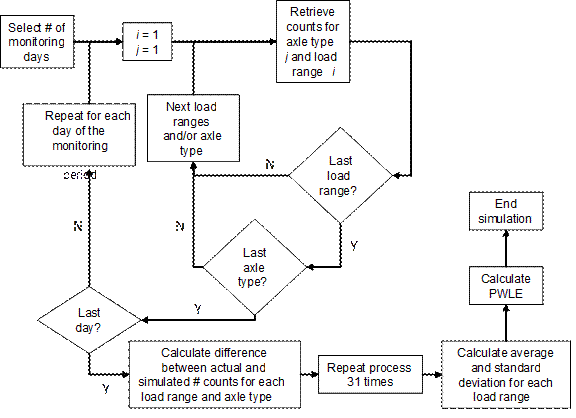
Figure 14. Flowchart. Monte Carlo simulation for analysis of data availability.

Example of Assessing the Impact of Daily Data Availability on Monthly NALS Estimate

The following example demonstrates the procedure used to evaluate PWLE associated with different data availability scenarios for a selected WIM site. Monte Carlo simulation was used to simulate different WIM data availability scenarios, expressed as number of consecutive days of data collection within a month. For this example, no precision or bias errors were simulated, and the objective was to evaluate the impact of the sample size (number of monitoring days) on the reliability of monthly axle load spectrum estimates.

To select a site for this analysis, monthly variability of tandem axle overloads was evaluated for all sites, months, and SPS TPF years. A site that had representative high monthly variability in overloads and availability of full month of daily data was selected for this example (site 20-0200 for July 2008).

Figure 15 shows the results of PWLE computation associated with different data availability scenarios simulated using 1 month of data. In this case, 31 days of data were available for the month, and the measured counts were assumed to be the actual daily counts for the site. The Monte Carlo technique was used to simulate the outcome of the load spectra when variable number of consecutive monitoring days was used. As expected, PWLE decreased as the number of monitoring days increased, and the drop in error was very significant when at least 5 monitoring days were available. In this example, it is evident that an increase in the number of available monitoring days beyond 7 DOW produced relatively low improvement in PWLE. This finding is further investigated in chapter 6 of this report.

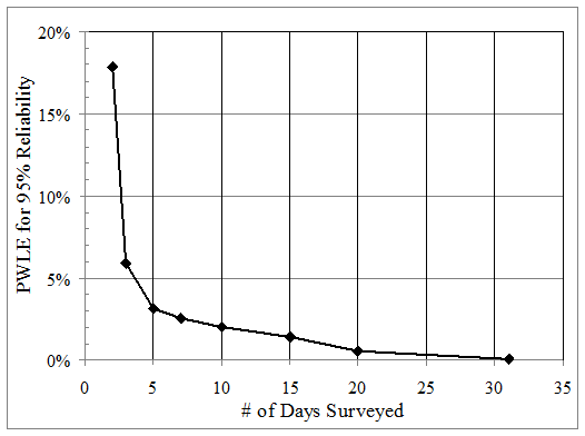
Figure 15. Graph. Impact of number of monitoring days on PWLE for site 20-0200.

Procedure to Assess the Impact of WIM Precision and Bias

The Monte Carlo simulation steps used in the analysis is a variation of that described in the previous example. Figure 12 is a flowchart that summarizes the flow of calculations for the simulation used in this example. The following procedure shows the steps involved in the Monte Carlo simulation:

1. Select number of consecutive days of data collection (7 or 31 days) to run the simulation.
   
   
   1. Randomly select the first monitoring day from the month.
      
      
   2. Retrieve the number of counts in each load bin from the database for each selected day for each axle group type.
      
      
   3. Randomly generate a load for every count in the load bin based on a uniform distribution between the minimum and maximum loads that define a given load bin.
      
      
   4. Adjust the load value from step iii for equipment precision and bias.
      
      
      1. Generate a random load magnitude to simulate precision error based on a normal distribution with the mean equal to the above random load and a random error based on the user-defined limit error for the axle group type (the following limits were obtained from SPS TPF data analysis: 8.9 percent for single axles and 7.7 percent for other axle group types with a 95 percent level of confidence).
         
         
      2. Multiply the load obtained in step iii to simulate bias error by 1 ±0.039 for positive/negative bias of single axles or 1 ±0.035 for positive bias of tandem, tridem, and quad axles (these values were obtained from SPS TPF data analysis; different values could be used to simulate different bias).
         
         
   5. Assign the randomly generated load to the corresponding load bin.
      
      
   6. Repeat steps iii to v until each count in the load bin has been simulated.
      
      
   7. Repeat steps ii to vi until all the load bins are exhausted.
      
      
   8. Repeat ii to vii until all axle group types are exhausted.
      
      
   9. Repeat steps from i to viii for the next day in the month until all consecutive survey dates are exhausted.
      
      
2. Save the simulated load spectrum.
   
   
3. Calculate and save the difference in load counts between the actual and the simulated counts as percent error of the counts in each load bin.
   
   
4. Repeat the selection of the first monitoring day of the month and development of spectrum based on precision and bias for 1,000 simulations. Although the simulation involves selection of the same day for multiple runs, each of these runs will be different due to the error associated with WIM precision and bias.
   
   
5. Compute the PWLE for 95 percent confidence as function of the number of monitoring days during the month. PWLE is the maximum expected error for the scenario.
   
   
6. Select a different number of days of data collection and repeat the process from steps 1 through 5.

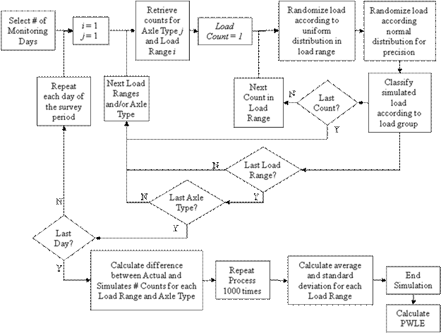
Figure 16. Flowchart. Monte Carlo simulation for analysis of precision and bias.

Procedure to Assess Reliability of Annual NALS Estimates

The procedure to calculate PWLE associated with representative annual normalized axle load spectra (RANALS) for an individual site takes into account the process used to compute annual NALS. The computation requires a minimum of 12 months of WIM data (each calendar month, January through December) for which at least 7 days of data (each DOW, Monday through Sunday) are available for each month to mitigate potential seasonal and DOW biases.

The load spectra computed for each of the 12 months of the year (all vehicle classes combined) are used to calculate the average percentage of axle loads in the annual NALS by averaging monthly axle load percentages P_ij for load bin i and axle group type j. In addition to the average value for each load bin, the variance is calculated based on the 12 monthly values for each load bin, and both parameters are used to calculate PWLE for the site. Assuming the deviations in percent axle loads for a given load bin in the spectrum have a normal distribution, the range of error can be estimated for a desired CL. In this case, the PWLE formula takes the following form in figure 17.

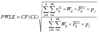
Figure 17. Equation. PWLE representing the whole axle load spectrum.

Where:

PWLE = Represents the whole axle load spectrum (all vehicle classes and axle group types combined) of an individual site.

W_{ij =} Weight (RPPIF) for load bin i and axle group type j developed in this study based on MEPDG sensitivity analysis (see table 4).

CF = Depends on the desired CL for the error, assuming the error is normally distributed; for 95 percent CL, CF is equal to 1.96 (see table 6).

i = Load bin.

j = Axle group type.

nb_i = Number of load bins for axle group type i.

p_j = Percentage of total axles corresponding to axle group type j computed using data for the 12 months.

= Average percentage of axle loads in the annual normalized axle load spectrum computed by averaging 12 monthly axle load percentages P_ij for load bin i and axle group type j.

v_if¹² = Variance of axle load percentages P_ij in the annual normalized axle load spectrum for load bin i and axle group type j computed using 12 monthly axle load percentages P_ij for load bin i and axle group type j.

It should be noted that CF presented in table 6 represents population values rather than studentt-value factors for a sample used in table 5. This is a simplification, since all 12 months of data are used to estimate the annual load spectrum. Also, the values in table 6 should be used to calculate PWLE for a given month if axle load data are available for the whole month. For any other case, table 5 values should be used in the PWLE formula, particularly when calculating PWLE for default spectra based on a certain sample of n sites.

The variance v_if¹² for a given load bin i and axle group type j is calculated based on the percentages of axle counts in that load bin for the 12 individual monthly estimates. For example, if the percentage of tandem axle loads between 30,000 and 31,999 lb are 4, 6, 7, 6, 5, 3, 7, 4, 5, 6, 6, and 3 percent (corresponding to the months from January to December), the variance (computed as the average of the squared differences from the mean value) is 2 percent.

The following steps should be used to calculate PWLE:

1. Select WIM site for analysis that satisfies minimum data availability requirements (12 calendar months with at least 7 DOW of data per month).
   
   
2. Compute NALS (all classes combined) for each axle group type, for each of the 12 months for the selected site. This will provide percentage of axle counts P_ij for each load bin i and axle group type j.
   
   
3. Compute total annual number and percentage of axles (p_j) for each axle group type.
   
   
4. Compute averageand associated variance v_if¹² for each load bin i and axle group type j. This is done based on the percentages of axle counts P_ij in each load bin i using data from the 12 individual monthly estimates.
   
   
5. Select desired CL.
   
   
6. Obtain CF based on selected CL from table 6.
   
   
7. Obtain W_ij factors from table 4 for each axle group type.
   
   
8. Compute PWLE using the formula presented above.

The calculation of PWLE associated with representative annual NALS estimate for individual sites is based on the monthly variance (of percent counts obtained for load bins). It can be argued that this monthly variance arises primarily from seasonal or monthly effects rather than WIM system errors. However, the monthly estimates from WIM data used in computation of variance for PWLE incorporate all sources of error as well as daily traffic data variation. Therefore, by using the monthly variances, the overall error associated with WIM data is assessed. One exception is WIM system bias. If a WIM system has a consistent bias that is not mitigated/changed between calibration visits, this bias is not accounted for in PWLE estimation for individual sites.

Example of Assessing Reliability of Annual NALS Estimates

An example PWLE calculation associated with annual NALS estimate for an individual site is presented in this section. Data for site 51-0100 were used in this example. Table 7 presents the distribution of axle counts by axle group type based on 30 months of data for this site.

Figure 18 presents the RANALS by axle group type for the site.

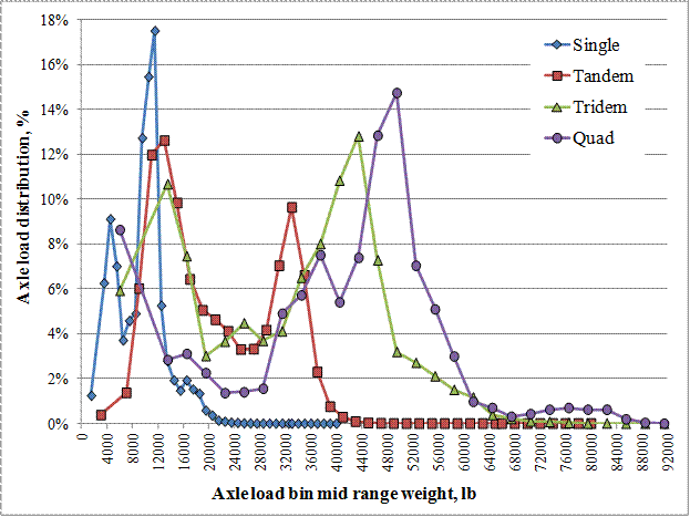
Figure 18. Graph. RANALS by axle group type.

RANALS were computed using the 12 monthly spectra estimates (one for each calendar month) and axle group type. If data for more than 1 year were available for a given calendar month, the average monthly percentages based on multiple years for each load bin were computed to characterize the spectrum for that month.

Averagesand variancesv_if¹² of the percentages for each load bin i and axle group type j were computed based on the percentages of axle counts P_ij in each load bin using data from the 12 representative monthly estimates.

Weight factors (see table 4) were used as multipliers to account for the relative importance of the load bin in relation to pavement performance.

Using the averages and variances for each load bin and axle group type over 12 months, PWLE for a desired CL was estimated based on monthly variability of axle load spectra, using the equation presented earlier. CF is obtained from table 6 (e.g., for 95 percent confidence, CF is 1.96).

For the example presented here, PWLE for the 95 percent confidence was found to be 1.27 percent-a small value reflecting a site with small monthly variations in load spectra. This means that the representative error associated with percentages of axles reported in load bins comprising the annual NALS for the site is within ±1.27 percent for 95 percent of the observations.

It is important to note that it was assumed that WIM calibration procedures conducted for this site resulted in unbiased load measurements. Analysis of WIM calibration data for this site indicated that average bias for the monitoring period included in this analysis was -0.63 percent for the single axles, +1.83 percent for tandem axles, and +1.2 percent for GVW, as measured by calibration trucks. However, measurements obtained during calibration visits provide only a snapshot of equipment performance and reflect measurements associated with calibration trucks only. As such, these values cannot be used directly in the assessment of data reliability. Indirectly, drifts and changes associated with WIM bias are accounted for in computation of monthly axle load spectra and associated variance used in PWLE computation.

APPLICABILITY AND USABILITY OF RELIABILITY PROCEDURES DEVELOPED IN THIS STUDY

Applicability of Reliability Procedures

The statistical analysis approach to evaluate reliability of axle load spectra estimates presented in this chapter can be used to aid in the development of the data selection criteria for generating NALS defaults. It could be used to quantify the relative importance of various sources of errors in the characterization of axle load spectra. The main component of the proposed analysis is the computation of PWLE, a parameter that can be used to represent the reliability of the axle load spectrum for pavement design.

In addition to this study, States may choose to use the PWLE statistic and analytical approaches presented in this chapter to evaluate the reliability of their axle loading data and use this information for selecting their WIM data for development of MEPDG traffic inputs, including traffic loading defaults.

Other uses of PWLE include the following:

• Evaluation of load spectra reliability as a function of the number of monitoring days in a given month or the number of months of available data for a given site.
  
  
• Evaluation of the effect of different WIM performance characteristics (precision and bias) on reliability of NALS estimates.
  
  
• Evaluation of the effect of different WIM site conditions and WIM technology used on reliability of NALS estimates.
  
  
• Evaluation of the differences in variability/reliability of NALS estimates using data before and after WIM system calibration.

The procedure to assess the reliability of axle load spectrum estimates using PWLE may be used for other applications as well. For example, it can be used to assess the representative error when a different number of sites with WIM data are used to estimate the load spectrum for a roadway section in the same region.

Recommended Future Development and Use of PWLE

PWLE is a new parameter introduced in this study, and additional studies may be required to determine acceptable PWLE levels for different pavement design and analysis applications, as well as different MEPDG input levels (levels 1-3). These acceptable PWLE levels should be determined based on changes in pavement performance predictions or pavement design estimates to answer the question, how close is close enough? Higher accuracy levels of traffic inputs may be required for design of pavements of higher volume roads (i.e., roads of higher significance).