U.S. Department of Transportation
Federal Highway Administration
1200 New Jersey Avenue, SE
Washington, DC 20590
202-366-4000
Federal Highway Administration Research and Technology
Coordinating, Developing, and Delivering Highway Transportation Innovations
| REPORT |
| This report is an archived publication and may contain dated technical, contact, and link information |
|
| Publication Number: FHWA-HRT-17-104 Date: June 2018 |
Publication Number: FHWA-HRT-17-104 Date: June 2018 |
To demonstrate the multi-objective approach, a subset of the LTPP data from a specific region was selected for calibration of MEPDG permanent deformation (rutting) prediction models for new and rehabilitated flexible pavements.
This chapter discusses the extraction of relevant LTPP data, calculation of the necessary parameters, and selection of other necessary values for generating the AASHTOWare® Pavement ME Design software input files. Following the discussion of the region selection process according to data availability, the LTPP data extraction and calculation of the required general, performance, traffic, climate, and structure/materials values are discussed.
The following steps demonstrate the process used to narrow the search for a suitable set of LTPP sections to collect calibration data. The LTPP InfoPaveTM website has been very useful in filtering the relevant test sections and identifying the availability of the required data.(40)
Table 6. Available number of test sections for each LTPP climatic region and subgrade type.
| Coarse-Grained Subgrade | Sections | Fine-Grained Subgrade | Sections |
|---|---|---|---|
| Dry, freeze | 100 | Dry, freeze | 39 |
| Dry, no freeze | 122 | Dry, no freeze | 28 |
| Wet, freeze | 143 | Wet, freeze | 132 |
| Wet, no freeze | 259 | Wet, no freeze | 191 |
There are more options among sections on coarse-grained subgrade soils (624 test sections) than fine-grained subgrade soils (390) and within the wet climatic regions (725) compared to dry regions (289). Based on the number of test sections in table 6, the search was narrowed to sections in the wet, no freeze climatic region.
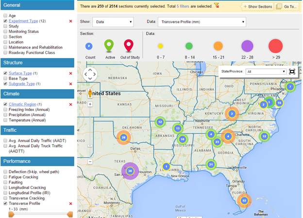
The InfoPaveTM map in figure 3 indicates the distribution of the 259 sections within the wet, no freeze climate and on coarse subgrades.(40) Most of these test sections are in Florida, Texas, Oklahoma, Georgia, and Alabama. The highest recorded amount of measured rut depth is between 22 and 28 mm (as indicated on the map).
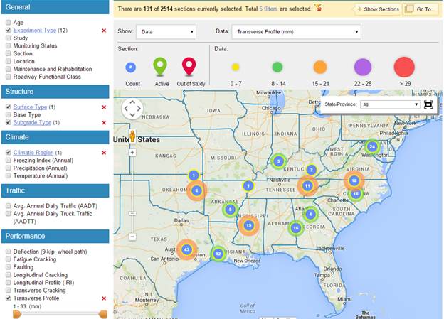
The InfoPaveTM map in figure 4 shows the distribution of the 191 sections within the wet, no freeze climate and on fine subgrades.(40) The majority of these test sections are located in Texas, Maryland, Mississippi, and Virginia, in that order. The highest recorded amount of measured rut depth is between 15 and 21 mm (as indicated on the map).
From the InfoPaveTM maps, it seems Florida has the highest number (52) of eligible test sections to be used for this study.(40) In addition to the results of this preliminary evaluation being in favor of selecting the Florida region for this project, FDOT has offered the flexible pavement data collected at their APT facility to be used in this study. The eligible LTPP test sections in Florida and the corresponding general information are listed in table 7. The LTPP Standard Data Release (SDR) number 29.0 was used for identifying the available data for this study.(40) The LTPP Information Management System (IMS) User Guide was used to identify the relevant sources (tables and fields) of data.(41)
Source: FHWA.
Figure 3. Screenshot. Location of sections within the wet, no freeze climate and on coarse subgrades from InfoPaveTM.
Source: FHWA.
Figure 4. Screenshot. Location of sections within the wet, no freeze climate and on fine subgrades from InfoPaveTM.
Table 7. General information on the 52 flexible test sections on coarse subgrade soils in Florida.
| # | STATE CODE |
SHRP ID |
Highway | Direction | EXPERIMENT TYPE |
CONST DATE |
OL_DATE | END_DATE | NEW_OR OVERLAY |
BASE TYPE |
|---|---|---|---|---|---|---|---|---|---|---|
| 1 | 12 | 0101 | US-27 | South | SPS-1 | 3/8/1995 | N/A | 7/13/2012 | New | GB |
| 2 | 12 | 0102 | US-27 | South | SPS-1 | 3/7/1995 | N/A | 7/13/2012 | New | GB |
| 3 | 12 | 0103 | US-27 | South | SPS-1 | 3/7/1995 | N/A | 7/13/2012 | New | ATB |
| 4 | 12 | 0104 | US-27 | South | SPS-1 | 3/7/1995 | N/A | 7/13/2012 | New | ATB |
| 5 | 12 | 0105 | US-27 | South | SPS-1 | 3/7/1995 | N/A | 7/13/2012 | New | GB |
| 6 | 12 | 0106 | US-27 | South | SPS-1 | 11/20/1995 | N/A | 7/13/2012 | New | GB |
| 7 | 12 | 0107 | US-27 | South | SPS-1 | 5/1/1995 | N/A | 7/13/2012 | New | GB |
| 8 | 12 | 0108 | US-27 | South | SPS-1 | 5/2/1995 | N/A | 7/13/2012 | New | GB |
| 9 | 12 | 0109 | US-27 | South | SPS-1 | 3/7/1995 | N/A | 7/13/2012 | New | GB |
| 10 | 12 | 0110 | US-27 | South | SPS-1 | 11/20/1995 | N/A | 7/13/2012 | New | ATB |
| 11 | 12 | 0111 | US-27 | South | SPS-1 | 11/20/1995 | N/A | 7/13/2012 | New | ATB |
| 12 | 12 | 0112 | US-27 | South | SPS-1 | 11/28/1995 | N/A | 7/13/2012 | New | ATB |
| 13 | 12 | 0161 | US-27 | South | SPS-1 | 3/3/1995 | N/A | 7/13/2012 | New | GB |
| 14 | 12 | 0502 | US-1 | South | SPS-5 to GPS-6S | 4/1/1971 | 4/18/1995 | 7/24/2014 | Overlay | GB |
| 15 | 12 | 0503 | US-1 | South | SPS-5 to GPS-6S | 4/1/1971 | 4/18/1995 | 7/24/2014 | Overlay | GB |
| 16 | 12 | 0504 | US-1 | South | SPS-5 to GPS-6S | 4/1/1971 | 4/18/1995 | 7/24/2014 | Overlay | GB |
| 17 | 12 | 0505 | US-1 | South | SPS-5 to GPS-6S | 4/1/1971 | 4/18/1995 | 7/24/2014 | Overlay | GB |
| 18 | 12 | 0506 | US-1 | South | SPS-5 to GPS-6S | 4/1/1971 | 4/18/1995 | 7/24/2014 | Overlay | GB |
| 19 | 12 | 0507 | US-1 | South | SPS-5 to GPS-6S | 4/1/1971 | 4/18/1995 | 7/24/2014 | Overlay | GB |
| 20 | 12 | 0508 | US-1 | South | SPS-5 to GPS-6S | 4/1/1971 | 4/18/1995 | 7/24/2014 | Overlay | GB |
| 21 | 12 | 0509 | US-1 | South | SPS-5 to GPS-6S | 4/1/1971 | 4/18/1995 | 7/24/2014 | Overlay | GB |
| 22 | 12 | 0561 | US-1 | South | SPS-5 to GPS-6S | 4/1/1971 | 4/18/1995 | 7/24/2014 | Overlay | GB |
| 23 | 12 | 0562 | US-1 | South | SPS-5 to GPS-6S | 4/1/1971 | 4/18/1995 | 7/24/2014 | Overlay | GB |
| 24 | 12 | 0563 | US-1 | South | SPS-5 to GPS-6S | 4/1/1971 | 4/18/1995 | 7/24/2014 | Overlay | GB |
| 25 | 12 | 0564 | US-1 | South | SPS-5 to GPS-6S | 4/1/1971 | 4/18/1995 | 7/24/2014 | Overlay | GB |
| 26 | 12 | 0565 | US-1 | South | SPS-5 to GPS-6S | 4/1/1971 | 4/18/1995 | 7/24/2014 | Overlay | GB |
| 27 | 12 | 0566 | US-1 | South | SPS-5 to GPS-6S | 4/1/1971 | 4/18/1995 | 7/24/2014 | Overlay | GB |
| 28 | 12 | 0901 | I-10 | East | SPS-9O | 6/1/1963 | 7/23/1996 | 5/15/2008 | Overlay | GB |
| 29 | 12 | 0902 | I-10 | East | SPS-9O | 6/1/1963 | 7/24/1996 | 5/15/2008 | Overlay | GB |
| 30 | 12 | 0903 | I-10 | East | SPS-9O | 6/1/1963 | 7/23/1996 | 5/15/2008 | Overlay | GB |
| 31 | 12 | 0959 | I-10 | East | SPS-9O | 6/1/1963 | 7/24/1996 | 5/15/2008 | Overlay | GB |
| 32 | 12 | 1030 | US-1 | South | GPS-1 to 6S | 4/1/1971 | N/A | 7/24/2014 | N/A | GB |
| 33 | 12 | 1060 | SH-878 | West | GPS-1 | 10/1/1979 | N/A | 3/7/2003 | N/A | GB |
| 34 | 12 | 1370 | SH-407 | North | GPS-1 to 6S | 6/1/1973 | 8/15/2000 | 4/24/2015 | Overlay | GB |
| 35 | 12 | 3995 | I-95 | North | GPS-1 | 12/1/1975 | N/A | 4/17/1997 | N/A | GB |
| 36 | 12 | 3996 | US-19 | North | GPS-1 | 4/1/1974 | N/A | 6/1/1998 | N/A | GB |
| 37 | 12 | 3997 | US-17 | South | GPS-1 to 6S | 6/1/1974 | 2/7/1995 | 7/13/1999 | Overlay | GB |
| 38 | 12 | 4096 | SH-20 | West | GPS-2 to GPS-6C | 5/1/1974 | 2/21/2003 | N/A | Overlay | ATB |
| 39 | 12 | 4097 | I-10 | East | GPS-2 | 1/1/1986 | N/A | 1/15/2005 | N/A | CTB |
| 40 | 12 | 4099 | SH-884 | West | GPS-1 | 6/1/1976 | N/A | 6/29/1992 | N/A | GB |
| 41 | 12 | 4100 | SH-85 | North | GPS-2 to GPS-6S | 8/1/1976 | 8/29/2002 | 8/12/2012 | Overlay | ATB |
| 42 | 12 | 4101 | SH-528 | East | GPS-1 to 6B | 5/1/1967 | 7/31/1991 | 8/28/1996 | Overlay | GB |
| 43 | 12 | 4103 | SH-836 | West | GPS-1 | 6/1/1982 | N/A | 6/22/2000 | N/A | GB |
| 44 | 12 | 4105 | SH-9A | North | GPS-1 | 12/1/1984 | N/A | 6/3/1993 | N/A | GB |
| 45 | 12 | 4106 | I-95 | North | GPS-1 to 6S | 8/1/1987 | 11/15/2003 | 11/24/2009 | Overlay | GB |
| 46 | 12 | 4107 | SH-70 | West | GPS-1 | 10/1/1983 | N/A | 5/4/1998 | N/A | GB |
| 47 | 12 | 4108 | SH-30 | West | GPS-2 | 6/1/1986 | N/A | 10/25/1996 | N/A | ATB |
| 48 | 12 | 4135 | US-27 | North | GPS-1 to 6B | 2/1/1971 | 2/15/1992 | 6/12/2006 | Overlay | GB |
| 49 | 12 | 4136 | US-27 | North | GPS-1 to 6B | 2/1/1971 | 2/15/1992 | 6/12/2006 | Overlay | GB |
| 50 | 12 | 4137 | US-27 | North | GPS-1 to 6B | 12/1/1970 | 2/15/1992 | 6/12/2006 | Overlay | GB |
| 51 | 12 | 4154 | SH-442 | East | GPS-1 | 6/1/1970 | N/A | 3/31/1998 | N/A | GB |
| 52 | 12 | 9054 | SH-200 | West | GPS-1 | 10/1/1974 | N/A | 9/26/1997 | N/A | GB |
| SHRP_ID = Strategic Highway Research Program identification number; CONST_DATE = construction date; OL_DATE = overlay date; N/A = no adequate data; GB = granular base; ATB = asphalt-treated base; CTB = cement-treated base. | ||||||||||
The field named NEW_OR_OVERLAY in table 7 shows which test sections (13 sections total) were found most suitable for calibration of rutting prediction models for new pavements and which sections (27 sections total) were deemed more appropriate for calibration of rutting models for overlaid pavements. These selections were made based on the availability of monitoring data after original pavement construction or after overlay construction. In 12 test sections marked as N/A, there were not adequate data on maintenance and rehabilitation history before the sections were assigned to the LTPP program and monitored. Therefore, using the data from these 12 test sections is not recommended for the calibration process.
These test sections have adequate climatic data to be used. The AASHTOWare® Pavement ME Design software uses historical climate data (HCD) files, and each one of the LTPP sections do have a corresponding climate station in that database, which can be downloaded from the http://me-design.com/MEDesign/ClimaticData.html Web location. Recently, the LTPP program has also made Modern-Era Retrospective Analysis for Research and Applications (MERRA) data available since the SDR 29.0 and through the InfoPaveTM website.(40) In this research study, the original HCD files downloaded from the AASHTOWare® website were used as inputs. The next steps are exploring the amount of available traffic and structure data.
Table 8 shows the LTPP source tables and amount of available traffic data for the 52 test sections that met the selection criteria in Florida. The LTPP traffic (TRF) module contains tables that start with the TRF_MEPDG_ prefix. These tables contain traffic data estimated for input into the MEPDG software based on test sites that have more than 210 d of monitored data per year. However, for other site-years where the total number of accepted monitoring data was less than 210 d in that year, traffic data can still be found in the tables starting with the TRF_MONITOR_ prefix. As table 8 demonstrates, the majority of the test sections have some (for some years) traffic data available to be used in this study. The details of input data extraction and calculations are explained later in this chapter.
Table 9 shows the amount of available LTPP data for the most important structural factors. It was assumed that the material properties for one SPS section could be applied to other sections with the same material source within the same SPS site. The LTPP data field PROJECT_LAYER_NO in the tables starting with the TST prefix (the testing module, which contains the results of materials testing conducted under the LTPP program) was used to decide whether test results from one test section could be applied to other test sections within an SPS project site. It is noted that, due to construction variability, this might not be an accurate estimation, but it will be more representative of the field materials when compared to the MEPDG default values. The details of input data extraction and calculations are explained later in this chapter.
Table 8. Source and availability of traffic data for the selected 52 flexible sections in Florida.
| Data Item | LTPP Source Tables | Number of Sections With Available Data |
|---|---|---|
| AADTT | TRF_MEPDG_AADTT_LTPP_LN | 49 |
| AADTT | TRF_MONITOR_LTPP_LN | 52 |
| AADTT | TRF_HIST_EST_ESAL |
15 |
| AADTT | TRF_MON_EST_ESAL | 52 |
| Axle load distributions | TRF_MEPDG_AX_DIST_ANL | 31 |
| Axle load distributions | TRF_MONITOR_AXLE_DISTRIB | 52 |
| Number of axles per truck | Estimated based on data from TRF_MONITOR_LTPP_LN | 52 |
| Vehicle class distributions | TRF_MEPDG_VEH_CLASS_DIST | 49 |
| Vehicle class distributions | TRF_MONITOR_LTPP_LN | 52 |
| Monthly adjustment factors | TRF_MEPDG_MONTH_ADJ_FACTR | 49 |
| Hourly adjustment factors | TRF_MEPDG_HOURLY_DISTRIB | 28 |
| Traffic growth factor | Estimated based on data from TRF_MONITOR_LTPP_LN | 52 |
| Traffic growth function | Not available, assumed compound growth | N/A |
| LTPP lane, direction, and lane width | INV_GENERAL | 39 |
| LTPP lane, direction, and lane width | SPS_ID | 13 |
| Lane and directional distribution | Not directly available, both assumed to be 1.0 for calibration purposes | N/A |
| Operational speed | SECTION_GENERAL, not available for Florida sections | N/A |
| Tire pressure | Not available, MEPDG defaults | N/A |
| Axle configuration, wheelbase, and wheel location | Not available, MEPDG defaults | N/A |
| Truck wander | Not available, MEPDG defaults | N/A |
| AADTT = average annual daily truck traffic; N/A = no adequate data. | ||
Table 9. Source and availability of structure data for the selected 52 flexible sections in Florida.
| Data Item | LTPP Source Tables | Sections |
|---|---|---|
| Thickness of all layers | TST_L05B | 52 |
| Poisson’s ratio for all layers | Not available | MEPDG defaults |
| AC dynamic modulus | TST_AC07 | 34 |
| AC dynamic modulus | TST_ESTAR estimated values | 40 |
| AC air voids | For SPS-9: TST_SP02 | 4 |
| AC air voids | Other than SPS-9: TST_AC02 + TST_AC03 | 37 |
| AC effective binder volume | For SPS-9: TST_SP02 | 4 |
| AC effective binder volume | Other than SPS-9: TST_AC03 + TST_AC04 + TST_AG01 + TST_AG02 | 23 to 37 |
| AC shortwave absorptivity | Not available | MEPDG defaults |
| AC PG grading | LTPP Bind Online | 43 |
| AC heat capacity | Not available | MEPDG defaults |
| AC thermal conductivity | Not available | MEPDG defaults |
| Base resilient modulus | TST_UG07_SS07_WKSHT_SUM | 38 |
| Subgrade resilient modulus | TST_UG07_SS07_WKSHT_SUM | 38 |
| Subgrade percent passing no. 200 | TST_SS01_UG01_UG02 | 39 |
| Subgrade Atterberg limits | TST_UG04_SS03 | 39 |
In this section, it was determined that there are adequate structure–climate–traffic data in the LTPP database for some of the selected test sections to be used in calibration of rutting prediction models for the new and rehabilitated flexible pavements. However, the final data element is the performance monitoring data. Table shows the availability of the rutting measurements for the selected LTPP test sections in Florida. This table shows the rutting data only for the 40 test sections that were assigned to calibration of new (13 sections) or rehabilitated (27 sections) performance models in table 7.
Table 10. Availability of rutting data for the selected LTPP flexible pavements in Florida.
| # | STATE_ CODE |
SHRP_ ID |
EXPERIMENT_ TYPE |
NEW_OR_ OVERLAY |
BASE_ TYPE |
FIRST_RUT_ DATE |
LAST_RUT_ DATE |
NUMBER_RUT_ MEASUREMENT |
|---|---|---|---|---|---|---|---|---|
| 1 | 12 | 0101 | SPS-1 | New | GB | 2/9/2000 | 3/29/2011 | 12 |
| 2 | 12 | 0102 | SPS-1 | New | GB | 2/9/2000 | 3/29/2011 | 12 |
| 3 | 12 | 0103 | SPS-1 | New | ATB | 2/9/2000 | 3/29/2011 | 12 |
| 4 | 12 | 0104 | SPS-1 | New | ATB | 2/9/2000 | 3/30/2011 | 12 |
| 5 | 12 | 0105 | SPS-1 | New | GB | 2/9/2000 | 3/29/2011 | 12 |
| 6 | 12 | 0106 | SPS-1 | New | GB | 2/9/2000 | 4/4/2011 | 12 |
| 7 | 12 | 0107 | SPS-1 | New | GB | 2/9/2000 | 4/4/2011 | 12 |
| 8 | 12 | 0108 | SPS-1 | New | GB | 2/9/2000 | 4/4/2011 | 12 |
| 9 | 12 | 0109 | SPS-1 | New | GB | 2/9/2000 | 3/30/2011 | 12 |
| 10 | 12 | 0110 | SPS-1 | New | ATB | 2/9/2000 | 4/4/2011 | 12 |
| 11 | 12 | 0111 | SPS-1 | New | ATB | 2/9/2000 | 3/30/2011 | 12 |
| 12 | 12 | 0112 | SPS-1 | New | ATB | 2/9/2000 | 3/30/2011 | 12 |
| 13 | 12 | 0161 | SPS-1 | New | GB | 2/9/2000 | 11/3/2006 | 10 |
| 14 | 12 | 0502 | SPS-5 to GPS-6S | Overlay | GB | 1/21/1996 | 10/1/2013 | 16 |
| 15 | 12 | 0503 | SPS-5 to GPS-6S | Overlay | GB | 1/21/1996 | 10/1/2013 | 16 |
| 16 | 12 | 0504 | SPS-5 to GPS-6S | Overlay | GB | 1/21/1996 | 4/1/2011 | 15 |
| 17 | 12 | 0505 | SPS-5 to GPS-6S | Overlay | GB | 1/21/1996 | 10/3/2013 | 16 |
| 18 | 12 | 0506 | SPS-5 to GPS-6S | Overlay | GB | 1/21/1996 | 10/2/2013 | 16 |
| 19 | 12 | 0507 | SPS-5 to GPS-6S | Overlay | GB | 1/21/1996 | 10/2/2013 | 16 |
| 20 | 12 | 0508 | SPS-5 to GPS-6S | Overlay | GB | 1/21/1996 | 10/1/2013 | 16 |
| 21 | 12 | 0509 | SPS-5 to GPS-6S | Overlay | GB | 1/21/1996 | 10/1/2013 | 16 |
| 22 | 12 | 0561 | SPS-5 to GPS-6S | Overlay | GB | 1/21/1996 | 10/1/2013 | 14 |
| 23 | 12 | 0562 | SPS-5 to GPS-6S | Overlay | GB | 1/21/1996 | 10/2/2013 | 14 |
| 24 | 12 | 0563 | SPS-5 to GPS-6S | Overlay | GB | 1/21/1996 | 10/2/2013 | 14 |
| 25 | 12 | 0564 | SPS-5 to GPS-6S | Overlay | GB | 1/21/1996 | 10/3/2013 | 14 |
| 26 | 12 | 0565 | SPS-5 to GPS-6S | Overlay | GB | 1/21/1996 | 10/1/2013 | 14 |
| 27 | 12 | 0566 | SPS-5 to GPS-6S | Overlay | GB | 1/21/1996 | 1/29/2014 | 15 |
| 28 | 12 | 0901 | SPS-9O | Overlay | GB | 7/25/1996 | 10/11/2006 | 8 |
| 29 | 12 | 0902 | SPS-9O | Overlay | GB | 7/25/1996 | 10/11/2006 | 8 |
| 30 | 12 | 0903 | SPS-9O | Overlay | GB | 7/25/1996 | 10/11/2006 | 8 |
| 31 | 12 | 0959 | SPS-9O | Overlay | GB | 7/25/1996 | 1/24/2004 | 7 |
| 32 | 12 | 1370 | GPS-1 to 6S | Overlay | GB | 10/29/2001 | 10/10/2013 | 7 |
| 33 | 12 | 3997 | GPS-1 to 6S | Overlay | GB | 1/25/1996 | 3/1/1999 | 2 |
| 34 | 12 | 4096 | GPS-2 to GPS-6C | Overlay | ATB | 10/23/2003 | 3/25/2014 | 5 |
| 35 | 12 | 4100 | GPS-2 to GPS-6S | Overlay | ATB | 10/2/2002 | 2/13/2012 | 4 |
| 36 | 12 | 4101 | GPS-1 to 6B | Overlay | GB | 4/14/1992 | 1/22/1996 | 3 |
| 37 | 12 | 4106 | GPS-1 to 6S | Overlay | GB | 1/20/2005 | 5/11/2009 | 3 |
| 38 | 12 | 4135 | GPS-1 to 6B | Overlay | GB | 3/10/1994 | 5/5/2004 | 9 |
| 39 | 12 | 4136 | GPS-1 to 6B | Overlay | GB | 3/10/1994 | 5/5/2004 | 9 |
| 40 | 12 | 4137 | GPS-1 to 6B | Overlay | GB | 3/10/1994 | 6/9/2006 | 9 |
Average measured rutting values across the entire length of each test section can be extracted from the LTPP table MON_T_PROF_INDEX_SECTION, and the individual rutting values measured at 50-ft intervals can be extracted from the LTPP table MON_T_PROF_INDEX_POINT.
In the previous section, the availability of LTPP data in the selected Florida region was explored. This section explains the details of LTPP data extraction and the required calculations and assumptions to generate inputs for the AASHTOWare® Pavement ME Design software version 2.2.(1) The required MEPDG data have been classified into the following groups: project information, performance criteria, traffic data, climate data, pavement structure and materials, and permanent deformation (rutting) data. The LTPP SPS-1 and SPS-5 sites in Florida were selected for demonstration of the novel approach in this study for calibration of the rutting models for new and overlaid pavements, respectively.
The software has an interface to enter general information for every design project (table 11). For calibration purposes, the significant information is the design life. The default value is 20 yr, but it is important to enter a design life that encompasses the available performance data to be able to calibrate the models to those data. As table 7 and table demonstrate, the latest rutting measurement date compared to the construction date of the original or overlay surface was on SPS-5 sections, and the surface age at the latest measurement date was 19 yr. Therefore, in this study, the default design life of 20 yr was found to be adequate for calibration.
Table 11. General project information.
| Data Item | LTPP Source Tables | Data Field/Value |
|---|---|---|
| Section ID | EXPERIMENT_SECTION | SHRP_ID |
| Project location | EXPERIMENT_SECTION | STATE_CODE |
| Design type | New pavement or overlay per table 10 | N/A |
| Pavement type | Flexible pavement | N/A |
| Design life (years) | 20 yr | N/A |
| Base construction year/month | EXPERIMENT_SECTION | CN_ASSIGN_DATE |
| Pavement construction year/month | EXPERIMENT_SECTION | CN_ASSIGN_DATE |
| Traffic opening year/month | EXPERIMENT_SECTION | ASSIGN_DATE |
The software has an interface to enter some performance criteria to be met by the specific pavement design (table 12). However, this information is not significant for the purpose of calibrating the performance models. Therefore, the default values were used for this study.
Table 12. Performance criteria.
| Data Item | LTPP Source Tables | Data Field/Value |
|---|---|---|
| Initial IRI (m/km) | MEPDG defaults | 1 |
| Terminal IRI (m/km) limit | MEPDG defaults | 2.7 |
| Terminal IRI (m/km) reliability | MEPDG defaults | 90 |
| AC top-down fatigue cracking (m/km) limit | MEPDG defaults | 378.8 |
| AC top-down fatigue cracking (m/km) reliability | MEPDG defaults | 90 |
| AC bottom–up fatigue cracking (%) limit | MEPDG defaults | 25 |
| AC bottom–up fatigue cracking (%) reliability | MEPDG defaults | 90 |
| AC thermal cracking (m/km) limit | MEPDG defaults | 189.4 |
| AC thermal cracking (m/km) reliability | MEPDG defaults | 90 |
| Permanent deformation—total pavement (mm) limit | MEPDG defaults | 19 |
| Permanent deformation—total pavement (mm) reliability | MEPDG defaults | 90 |
| Permanent deformation—AC-only (mm) limit | MEPDG defaults | 6 |
| Permanent deformation—AC-only (mm) reliability | MEPDG defaults | 90 |
| IRI = International Roughness Index. | ||
Table 8 lists the general availability of the required traffic data within the LTPP database. In this section, the details of traffic input data extraction and calculation are explained. Table 13 lists some of the data sources used for traffic inputs. The LTPP TRF module contains tables that start with the TRF_MEPDG_ prefix. These tables contain traffic data estimated for input into the MEPDG software based on test sites that have more than 210 d of monitored data per year. However, for other site-years where the total number of accepted monitoring data was less than 210 d in that year, traffic data can still be found in the tables starting with the TRF_MONITOR_ prefix.
Table 13. Traffic input data sources and default values.
| Data Item | LTPP Source Tables | Data Field/Default Value |
|---|---|---|
| Two-way AADTT | TRF_MONITOR_LTPP_LN | TRUCKS_LTPP_LN |
| Number of lanes | Not applicable | 1 |
| % of trucks in design direction | Not applicable | 100 |
| % of trucks in design lane | Not applicable | 100 |
| Operational speed (kph) | SECTION_GENERAL Not available for Florida sections |
SPEED_LIMIT Used 100 kph based on posted limit. |
| Traffic capacity cap | Not enforced | N/A |
| Average axle width (m) | MEPDG defaults | 2.59 |
| Dual tire spacing (mm) | MEPDG defaults | 305 |
| Tire pressure (single tire) (kPa) | MEPDG defaults | 827.4 |
| Tandem axle spacing (m) | MEPDG defaults | 1.31 |
| Tridem axle spacing (m) | MEPDG defaults | 1.25 |
| Quad axle spacing (m) | MEPDG defaults | 1.25 |
| Mean wheel location (mm) | MEPDG defaults | 460 |
| Traffic wander standard deviation (mm) | MEPDG defaults | 254 |
| Design lane width (m) | MEPDG defaults | 3.6576 |
| Average spacing of short axles (m) | MEPDG defaults | 3.66 |
| Average spacing of medium axles (m) | MEPDG defaults | 4.57 |
| Average spacing of long axles (m) | MEPDG defaults | 5.49 |
| Percent trucks with short axles | MEPDG defaults | 33 |
| Percent trucks with medium axles | MEPDG defaults | 33 |
| Percent trucks with long axles | MEPDG defaults | 34 |
| Vehicle class distribution (%) | TRF_MEPDG_VEH_CLASS_DISTOr TRF_MONITOR_LTPP_LN | Multiple fields in these tables are used. |
| Growth rate (%) by vehicle class | Estimated based on data from TRF_MONITOR_LTPP_LN | TRUCKS_LTPP_LN |
| Growth function | Compound growth was assumed. | Compound growth was assumed. |
| Monthly adjustment factors by vehicle class | TRF_MEPDG_MONTH_ADJ_FACTR | Multiple fields in these tables are used. |
| Hourly adjustment factors | MEPDG defaults were used. | MEPDG defaults were used. |
| Axles per truck for each vehicle class and axle group | Estimated based on data from TRF_MONITOR_LTPP_LN | Multiple fields in these tables are used. |
| Axle load distribution for every axle group | TRF_MEPDG_AX_DIST_ANLOr TRF_MONITOR_AXLE_DISTRIB | Multiple fields in these tables are used. |
The traffic inputs in the MEPDG software comprise two main interfaces. The first interface includes basic traffic information, axle configuration, lateral wander, vehicle class distribution and growth, monthly adjustment, and axles per truck; the second interface includes the axle load distributions for single, tandem, tridem, and quad axles.
A software routine called LTPP Pavement Loading User Guide (PLUG) had previously been developed based on Microsoft® Access to populate the input data required for axle load distributions in the second interface.(42) However, the LTPP PLUG does not populate other traffic data required for the first interface in the MEPDG software. Therefore, during the current project, a series of Visual Basic for Applications (VBA) macros were developed in an Microsoft® Excel platform to extract, calculate, and create Extensible Markup Language (XML) data files to be imported into the MEPDG software for the first traffic inputs interface. In this manner, all traffic input data were imported into the MEPDG software using the generated XML files from the VBA macro codes created in this project and from the LTPP PLUG software.
Within the basic traffic information, the initial two-way average annual daily truck traffic (AADTT) is the most significant information. In this study, the LTPP table TRF_MONITOR_LTPP_LN, which is based on Automatic Vehicle Classification (AVC) and WIM equipment, was used as the source of AADTT. The data field TRUCKS_LTPP_LN in this table gives an estimate of the annual number of trucks in each class based on AVC and WIM information. The sum of these values for every year gives an estimate of AADTT in the LTPP lane for that year. Since the objective of this study is calibration of performance models based on performance measurements within LTPP test sections, these AADTT estimates were used along with the assumption that all of the roadway traffic has passed through the LTPP lane. In other words, a 100-percent value was used for directional and lane adjustment factors.
In MEPDG, the flexible pavement response model only requires the load spectrum, tire contact pressure distributions, and areas of contact for traffic characterization (see page 3.3.42 of the final report for NCHRP Project 1-37A).(2) However, for the slab cracking prediction model, the axle configuration, traffic wander, and wheelbase are considered critical factors (see page KK-9 and KK-10 of appendix KK of the final report for NCHRP Project 1-37A).(2) Since the axle configuration, lateral wander, and wheelbase information are only used for analysis and design of jointed concrete pavements, the default software values were used for this study.
The vehicle class distribution is extracted from the LTPP table TRF_MEPDG_VEH_CLASS_DIST where available (for any site-year where more than 210 d of monitored data have been recorded) and estimated from the LTPP table TRF_MONITOR_LTPP_LN otherwise. To generate MEPDG input values, the annual class distributions were averaged among all years of available data.
Data from the TRUCKS_LTPP_LN field in the TRF_MONITOR_LTPP_LN table were used to estimate a traffic growth factor by each vehicle class. For every vehicle class in each site, the available data were used with linear interpolation to fill in the gaps between the final available year and the initial year (for which AADTT was input) and create a continuous series of truck counts. Then the initial counts and the final cumulative counts were used with an assumption of compound growth to estimate the growth factor r. In equation 20, Tf is the cumulative truck count for every class at the final year of available data, Ti is the truck count at the initial year, and Y is the difference in the number of years between the initial year and the final year of available data. Equation 20 was recursively solved using a VBA macro to estimate r, or growth factor, for every vehicle class:
 (20)
(20)
Where:
Tf = cumulative traffic at the end of the period.
Ti = traffic at the beginning of the period.
r = growth factor.
Y = period in years.
For monthly adjustment factors, data from the LTPP table TRF_MEPDG_MONTH_ADJ_FACTR were used. The LTPP TRF_MEPDG_HOURLY_DISTRIB has hourly adjustment factors only for the LTPP sites that were in the traffic pooled fund study. Since hourly distributions are more important in analysis of jointed concrete pavements, the MEPDG default values were used for hourly distributions in this study.
For every vehicle class, based on the estimated count of axles in each axle group (single, tandem, tridem, or quad) within the TRF_MONITOR_LTPP_LNtable, the number of axles per truck is calculated. This number is then averaged among all years with available data to generate the MEPDG inputs.
For each LTPP site-year with adequate data (more than 210 d of monitored data per year), the TRF_MEPDG_AX_DIST_ANL table was used to generate the MEPDG required inputs. For other site-years, data from the TRF_MONITOR_AXLE_DISTRIB table were converted to generate the corresponding MEPDG inputs. All of these data were reformatted to be input into the LTPP PLUG tables. Then the PLUG software was used to generate the required XML files for each site.
The AASHTOWare® Pavement ME Design software has two options to gather the climatic data—a single weather station or a virtual weather station. The appropriate option is selected based on the proximity of the section to a certain weather station. Existing weather stations (the data for which can be downloaded at http://me-design.com/MEDesign/ClimaticData.html) are listed by location and can be searched by latitude and longitude. The latitude and longitude data are available in table SECTION_COORDINATES of the LTPP database. Table 14 lists the data source and the corresponding fields.
Table 14. Climate information.
| Data Item | LTPP Source Tables | Data Field/Value |
|---|---|---|
| Longitude (degrees, minutes) | SECTION_COORDINATES | LONGITUDE |
| Latitude (degrees, minutes) | SECTION_COORDINATES | LATITUDE |
| Elevation (ft) | AWS_LOCATION | ELEVATION |
| Depth of water table (ft) | N/A | 5 m (+1) |
| Climate station | MEPDG | N/A |
| Note: (+1) a default value of 5 m was set for the depth of the water table, since this information is not available from the LTPP database. | ||
The LTPP InfoPave™ website has a tool for extracting the National Aeronautics and Space Administration MERRA climatic data in the form of HCD files for each LTPP test section.(40) This tool also provides the station information in the form of a station.dat file. These files can be copied to the climatic data folder, which has been designated by the user for the AASHTOWare® software.(1) This way, the user will also have the option to use MERRA climatic data. For the current project, only the existing weather station data were used.
Pavement layers are identified in LTPP with a unique number (LAYER_NO). Layer number 1 is always assigned to the lowest layer (subgrade) in the pavement structure, and additional layers above it are indicated with progressively larger layer numbers. In addition to LAYER_NO, which is specific to each test section, for the SPS projects, which have more than one test section per site, a layer identifier, PROJECT_LAYER_CODE, is available. Pavement layers with the same material properties from different test sections along the entire site are identified using this field code. Even though the sequence of a layer might be different in different test sections (different LAYER_NO), a similar PROJECT_LAYER_CODE indicates that those layers from different test sections were constructed at the same time and using similar materials.
Since not every section has test results for each layer, an expansion data process was applied to populate the layer structure properties. Under this process, the test results from one section are expanded to the other section when the PROJECT_LAYER_CODE in both sections is the same for a given layer. This process is applied to the entire site for the Florida SPS-1 and SPS-5 test sections.
Before applying the described procedure, sections need to be ordered according to the construction sequence (SECTION_START and SECTION_END fields in the SPS_PROJECT_STATIONS table). Then blank fields are filled with data available from the closest section having the same PROJECT_LAYER_CODE. The description of the layer was also taken into consideration for the expansion of subgrade test results.
Layer thickness and type of material are extracted from the LTPP table TST_L05B (SECTION_LAYER_STRUCTURE). Table 15 summarizes the data required for input into MEPDG software and the corresponding LTPP tables and fields.
Table 15. Layer thickness and type of material.
| Data Item | LTPP Source Tables | Data Field/Value |
|---|---|---|
| Thickness (mm) | TST_L05B, SECTION_LAYER_STRUCTURE | REPR_THICKNESS |
| Construction number | TST_L05B, SECTION_LAYER_STRUCTURE | CONSTRUCTION_NO |
| Layer number | TST_L05B, SECTION_LAYER_STRUCTURE | LAYER_NO |
| Type of material | TST_L05B, SECTION_LAYER_STRUCTURE | MATL_CODE |
| Material that is similar among SPS sections on one site | SECTION_LAYER_STRUCTURE | PROJECT_LAYER_CODE |
Wherever data were available, input level 1 was considered for the AC layer. Under this input level, binder properties, mixture volumetric properties, dynamic modulus, and creep compliance need to be provided according to laboratory test results. Mixture volumetric properties calculations were made using available LTPP test results prior to introducing the data into the software. Dynamic modulus master curve is calculated internally in the software when it is provided with the dynamic modulus for a combination of laboratory test results. Individual values for creep compliance are introduced, and the software calculates the master curve.
Mixture Volumetric Information
The mixture volumetric information was calculated with the LTPP data and applying the weight–volume relationships for asphalt mixtures.(43) Relevant values for the volumetric calculation were taken from LTPP TST tables as described in table 16.
Table 16. Mixture volumetric data.
| Data Item | LTPP Source Tables |
Data Field/Value |
|---|---|---|
| Unit weight (kg/m3) | TST_AC02 | BSG 1,000 |
| Effective binder content (%) | TST_AC04 | ASPHALT_CONTENT_MEAN (Pb = asphalt, percent by total weight of mixture) |
| Effective binder content (%) | TST_AC03 | MAX_SPEC_GRAVITY (Gmm = maximum SG of paving mixture) |
| Effective binder content (%) | TST_AG01 | BSG_OF_COARSE_AGG (Gsb = BSG of aggregate) |
| Effective binder content (%) | TST_AG02 | BSG_OF_FINE_AGG (Gsb = BSG of aggregate) |
| Air voids (%) | TST_AC02 | BSG (Gmb = BSG of compacted mixture) |
| Air voids (%) | TST_AC03 | MAX_SPEC_GRAVITY (Gmm = maximum SG of paving mixture) |
| BSG = bulk specific gravity. | ||
The following relationships were applied to calculate the effective binder content (equation 21) and the air voids (equation 26).
![]() (21)
(21)
Where:
Pbe = effective binder content (%).
Pb = asphalt, percent by total weight of mixture.
Pba = absorbed asphalt, percent by weight of aggregate, calculated using equation 22:
![]() (22)
(22)
Where Gse is the effective specific gravity (SG) of aggregate, calculated using equation 23:
 (23)
(23)
Where Gsb is the bulk specific gravity (BSG) of aggregate, calculated using equation 24:
 (24)
(24)
Where:
Pi = percentages by weight of aggregates.
Gi = BSG of aggregates.
Gb = asphalt SG, considered 1.01.(44)
Gmm = maximum SG of paving mixture, calculated using equation 25:
 (25)
(25)
Then the air voids are calculated with equation 26:
![]() (26)
(26)
Where:
Va = air voids (%).
Gmb = BSG of compacted mixture.
Binder and Asphalt Concrete Properties
Binder properties are available in the LTPP database, except for the softening point (table 17). This item is obtained indirectly by applying the correlation between temperature and viscosity, considering that the softening point value is associated uniquely with a viscosity of 13,000 poise.(45) Viscosity–temperature parameters correspond to MEPDG recommended values for an asphalt cement grade 40-50 (A = 10.5254 and VTS = –3.5047). Applying equation 27, the softening point temperature for the specified viscosity is 47 ºC.
![]() (27)
(27)
Where:
η = viscosity, centipoise (cP).
Tr = reference temperature, R.
A = regression intercept
VTS = regression slope or viscosity temperature susceptibility.
Table 17. Binder properties.
| Data Item | LTPP Source Tables | Data Field/Value |
|---|---|---|
| Poisson’s ratio | MEPDG defaults | MEPDG defaults |
| Softening point (ºC) at 1,300 pascal-sec | MEPDG defaults | 47 ºC |
| Absolute viscosity (pascal-sec) at 60 ºC | TST_AE_02 | ABSOLUTE_VISC_140_F |
| Kinematic viscosity (centistokes) at 135 ºC |
TST_AE_02 | KINEMATIC_VISC_275_F |
| SG at 25 ºC | TST_AE_03 | SPECIFIC_GRAVITY |
| Penetration at temperature 25 ºC | TST_AE_02 | PENETRATION_77_F |
AC dynamic modulus master curve is calculated internally in the MEPDG. This calculation is done based on the individual dynamic modulus values entered for a set of frequency and temperature combinations. The general expression for the dynamic modulus master curve is in equation 28:(1)
![]() (28)
(28)
Where:
t = time of loading at a given temperature of interest.
δ, α = fitting parameters; for a given set of data, δ represents the minimum value of E*, and δ + α represents the maximum value of E*.
β, γ = parameters describing the shape of the sigmodal function.
c = fitting parameter.
ηTr = viscosity at reference temperature.
It should be noted that the dynamic modulus values available within the LTPP TST_ESTAR_ tables have been calculated using an ANN model developed under a previous LTPP data analysis project. This ANN model uses actual laboratory-tested resilient modulus values available within the LTPP TST_AC07_ tables. Considering that calculated dynamic modulus values based on a relationship to the resilient modulus test results are used here, by MEPDG definition, this is level 2 input. However, the only option within the software to enter calculated dynamic modulus values was to use the level 1 input option. If the level 2 input option is selected, the software requires material properties other than the resilient modulus to predict the dynamic modulus based on the Witczak model.
Table 18 shows the LTPP tables and corresponding fields where the required input values regarding binder and mixture properties have been stored. In using the TST_ESTAR_ tables, the ESTAR_LINK corresponding to PREDICTIVE_MODEL number 1 was used, as the first predictive ANN model is the one estimating dynamic modulus based on resilient modulus lab testing results.
Table 18. Mixture properties.
| Data Item | LTPP Source Tables | Data Field/Value |
|---|---|---|
| Poisson’s ratio | MEPDG defaults | MEPDG defaults |
| Temperature levels for dynamic modulus | TST_ESTAR_MODULUS (TST_ESTAR_MASTER.PREDICTIVE_ MODEL = 1) which has been populated based on TST_AC07_V2_MR_SUM values |
TEMPERATURE |
| Frequency levels for dynamic modulus | TST_ESTAR_MODULUS (TST_ESTAR_MASTER.PREDICTIVE_ MODEL = 1) which has been populated based on TST_AC07_V2_MR_SUM values |
FREQUENCY |
| Dynamic modulus | TST_ESTAR_MODULUS (TST_ESTAR_MASTER.PREDICTIVE_ MODEL = 1) which has been populated based on TST_AC07_V2_MR_SUM values |
ESTAR |
| Creep compliance (1/GPa) | MEPDG defaults | MEPDG defaults |
| Thermal conductivity (watt/meter-kelvin) | MEPDG defaults | MEPDG defaults |
| Heat capacity (joule/kilogram-kelvin) | MEPDG defaults | MEPDG defaults |
| Thermal contraction | MEPDG defaults | MEPDG defaults |
SPS-5 sections are experiments with HMA overlays. For this type of pavement structures, the MEPDG requires the backcalculated elastic modulus or the results of a structural adequacy evaluation of the existing pavement. In all the sections, the backcalculated elastic modulus was obtained from the LTPP database. During the history of the LTPP program, two data analysis studies were conducted to backcalculate all of the FWD data. The most recent study was the LTPP Determination of In-Place Elastic Layer Modulus: Backcalculation Methodology and Procedure.(46) The latest backcalculated elastic modulus data became available since the SDR 29.0 and can be downloaded from the InfoPaveTM website.(40) The backcalculated elastic modulus along with the frequency and temperature are required in the MEPDG software for the overlay analysis. Table 19 shows the LTPP data tables and fields where the backcalculated moduli and the corresponding information can be found.
Table 19. LTPP data tables and fields for backcalculated moduli.
| Data Item | LTPP Source Tables | Data Field/Value |
|---|---|---|
| Backcalculated modulus averaged for each FWD pass | BAKCAL_MODULUS_SECTION_LAYER | AVG_MODULUS |
| Backcalculated layer | BAKCAL_MODULUS_SECTION_LAYER | BC_LAYER_NO |
| Corresponding LTPP layer number | BAKCAL_LAYER_LINK | LAYER_NO |
| FWD pass number | BAKCAL_MODULUS_SECTION_LAYER | FWD_PASS |
| Test date | BAKCAL_PASS | TEST_DATE |
| Temperature | BAKCAL_BASIN | SURFACE_TEMP |
| Frequency | N/A | 15 Hz |
| Gradation percent passing 3/4-inch sieve |
TST_AG04 | THREE_FOURTHS_PASSING |
| Gradation percent passing 3/8-inch sieve |
TST_AG04 | THREE_EIGHTHS_PASSING |
| Gradation percent passing Nº4 sieve | TST_AG04 | NO_4_PASSING |
| Gradation percent passing Nº200 sieve | TST_AG04 | NO_200_PASSING |
For the testing frequency, several studies have recommended a value of 1/2t where t is the period of the FWD load pulse and can be extracted from the FWD time history data that are available in the LTPP Ancillary Information Management System and can be downloaded through InfoPave™.(44,40) Based on an observation of several of the FWD time histories, it was decided that a value of 16 Hz corresponding to t = 0.03 s was suitable to use in this project. This value also coincides with the findings from several past studies.(48–50)
Some of the SPS-1 sections have asphalt-treated bases (ATBs) and permeable asphalt-treated bases. Those materials behave similarly to HMA concrete. So, LTPP source tables and fields are the same as the ones described for HMA.
The additional AC layer properties required by the software are listed in table 20.
Table 20. Additional AC layer properties.
| Data Item | LTPP Source Tables | Data Field/Value |
|---|---|---|
| Surface shortwave absorptivity | MEPDG defaults | 0.85 |
| Is endurance limit applied? | MEPDG defaults | False |
| Endurance limit (microstrain) | MEPDG defaults | 100 |
| Layer interface | MEPDG defaults | Full friction interface |
Unbound materials response is characterized by the resilient modulus calculated from the LTPP materials testing module data (TST_UG07_SS07_* tables). The representative resilient modulus was calculated according to the guidelines provided in the NCHRP Project 1-28A study, which found that the summary resilient modulus should be reported using equation 29 and calculated for the following stress states: σ3 = 5 psi and σ1 = 15 psi for aggregate base/subbase and σ3 = 2 psi and σ1 = 6 psi for subgrade soils.(51) The calculated resilient modulus values are listed in table 39 of appendix A.
![]() (29)
(29)
Where:
k1, k2, k3 = regression constants.
Pa= atmospheric pressure equal to 14.7 psi.
θ = bulk stress, calculated using equation 30:
![]() (30)
(30)
Where τoct is the octahedral shear stress, calculated using equation 31:
![]() (31)
(31)
Where σ1 and σ3 are the principal stresses.
Table 21 shows the LTPP source tables and fields for the required input data for unbound aggregate and subgrade soils materials properties.
Table 21. LTPP data sources for unbound materials properties.
| Data Item | LTPP Source Tables | Data Field/Value |
|---|---|---|
| Layer thickness (inches) | TST_L05B | REPR_THICKNESS |
| Poisson’s ratio | N/A | MEPDG defaults based on AASHTO soil classification |
| Coefficient of lateral earth pressure (Ko) | N/A | MEPDG defaults based on AASHTO soil classification |
| Resilient modulus (level 2) | N/A | Equation 29 |
| Average applied max axial stress | TST_UG07_SS07_WKSHT_ SUM |
APPLIED_MAX_AXIAL_STRESS_ AVG (σ1) |
| Confining pressure | TST_UG07_SS07_WKSHT_ SUM |
CON_PRESSURE (σ3) |
| Average resilient modulus | TST_UG07_SS07_WKSHT_ SUM |
RES_MOD_AVG (Mr) |
| Average applied cyclic stress | TST_UG07_SS07_WKSHT_ SUM |
APPLIED_CYCLIC_STRESS_AVG (Scyclic) |
| Average resilient strain | TST_UG07_SS07_WKSHT_ SUM |
RES_STRAIN_AVG (εr) |
| Percent passing 0.020 mm | TST_SS02_UG03 | HYDRO_02 |
| Percent passing # 200 | TST_SS01_UG01_UG02 | NO_200_PASSING |
| Percent passing # 80 | TST_SS01_UG01_UG02 | NO_80_PASSING |
| Percent passing # 40 | TST_SS01_UG01_UG02 | NO_40_PASSING |
| Percent passing # 10 | TST_SS01_UG01_UG02 | NO_10_PASSING |
| Percent passing # 4 | TST_SS01_UG01_UG02 | NO_4_PASSING |
| Percent passing 3/8" | TST_SS01_UG01_UG02 | THREE_EIGHTHS_PASSING |
| Percent passing 1/2" | TST_SS01_UG01_UG02 | ONE_HALF_PASSING |
| Percent passing 3/4" | TST_SS01_UG01_UG02 | THREE_FOURTHS_PASSING |
| Percent passing 1" | TST_SS01_UG01_UG02 | ONE_PASSING |
| Percent passing 1 1/2" | TST_SS01_UG01_UG02 | ONE_AND_HALF_PASSING |
| Percent passing 2" | TST_SS01_UG01_UG02 | TWO_PASSING |
| Percent passing 3" | TST_SS01_UG01_UG02 | THREE_PASSING |
| Liquid Limit | TST_UG01_SS03 | LIQUID_LIMIT |
| Plasticity Index | TST_UG01_SS03 | PLASTICITY_INDEX |
| AASHTO soil classification | TST_AG04 | NO_10_PASSING |
| AASHTO soil classification | TST_SS01_UG01_UG02 | NO_4_PASSING and NO_200_PASSING |
| AASHTO soil classification | TST_UG01_SS03 | PLASTIC_LIMIT and PLASTICITY_INDEX |
| Maximum dry unit weight (pcf) | N/A | MEPDG defaults based on AASHTO soil classification |
| Saturated hydraulic conductivity (m/hr) | N/A | MEPDG defaults based on AASHTO soil classification |
| Specify gravity of soils (Gs) | N/A | MEPDG defaults based on AASHTO soil classification |
| Optimum gravimetric water content (%) | N/A | MEPDG defaults based on AASHTO soil classification |
| Soil water characteristic curve parameter (af, bf, cf, hr) | N/A | MEPDG defaults based on AASHTO soil classification |
| N/A = no adequate data. | ||
The AASHTOWare® Pavement ME Design software does not allow an ATB layer directly on top of the subgrade. Therefore, the subgrade was split into two layers with the same materials, each one with half the subgrade thickness.
For the Florida SPS-1 site, the pavement structure is supported by a compacted limerock embankment. The construction report indicated a hard material underneath the embankment that, for the modeling purposes, was considered as bedrock with the properties noted in table 22.
Table 22. Bedrock material properties.
| Data Item | LTPP Source Tables | Data Field/Value |
|---|---|---|
| Layer thickness | MEPDG defaults | Semi-infinite |
| Unit weight | MEPDG defaults | 2,240 |
| Poisson’s ratio | MEPDG defaults | 0.15 |
| Elastic modulus | MEPDG defaults | 5,171 |
Backcalculated values of resilient modulus are applied when laboratory results are not available. These backcalculated values need to be adjusted to laboratory conditions to use in ME design. The adjustment to laboratory condition is done internally by the software according to the selected C-value that is listed in table 23.(52)
Table 23. C-values to convert the backcalculated layer modulus values to an equivalent resilient modulus measured in laboratory.
| Layer Type | Location | C-value of Mr/EFWD Ratio |
|---|---|---|
| Aggregate base/subbase | Between a stabilized and HMA layer | 1.43 |
| Aggregate base/subbase | Below a PCC layer | 1.32 |
| Aggregate base/subbase | Below an HMA layer | 0.62 |
| Subgrade/embankment | Below a stabilized subgrade/embankment | 0.75 |
| Subgrade/embankment | Below an HMA or PCC layer | 0.52 |
| Subgrade/embankment | Below an unbound aggregate base | 0.35 |
| PCC = portland cement concrete. | ||
During each LTPP manual distress survey, the transverse profile of the pavement sections is measured at every 50 ft, which results in rutting measurements for both wheelpaths at 11 test locations across the length of each test section. Point-by-point rutting measurements and calculated average section rutting values are stored in the LTPP database. Table 24 shows the LTPP data source for rutting measurements.
Table 24. LTPP data source for rutting measurements (wire reference method).
| Data Item | LTPP Source Tables | Data Field/Value |
|---|---|---|
| Measurement date | MON_T_PROF_INDEX_SECTION MON_T_PROF_INDEX_POINT |
SURVEY_DATE |
| Average section left wheelpath rutting | MON_T_PROF_INDEX_SECTION | LLH_DEPTH_WIRE_REF_MEAN |
| Average section right wheelpath rutting | MON_T_PROF_INDEX_SECTION | RLH_DEPTH_WIRE_REF_MEAN |
| Point-by-point left wheelpath rutting | MON_T_PROF_INDEX_POINT | LLH_DEPTH_WIRE_REF |
| Point-by-point right wheelpath rutting | MON_T_PROF_INDEX_POINT | RLH_DEPTH_WIRE_REF |
Rutting measurements used to be conducted using a 1.8-m straightedge and a reference wire. Later, the LTPP program adopted the Face Dipstick device, which measures the transverse profile elevations at every foot along the width of the lane. Even after using the Dipstick, the rutting values have been recorded according to a simulated straightedge and the wire reference methods. There has been no concrete evidence as to which method produces a more repeatable or representative rutting measurement. In this study, the values recorded according to the wire reference method have been used as measured rutting values to be used in the calibration of permanent deformation models. In the wire reference method, the maximum displacement between the reference wire line and pavement surface is calculated in the left- and right-lane halves. Reference wire is placed at profile end points and connects peaks, which protrude above horizontal datum end points, with straight lines. Displacement is computed perpendicular to horizontal datum between end points.
Pavement permanent deformation is the result of incremental deformation in each layer of the pavement. MEPDG calculates the incremental deformation for each subseason at the mid-depth of each sublayer within the pavement system. Each layer contributes to the total permanent deformation according to its material properties, climate, and load conditions. The rutting measurements in the LTPP database are for the total pavement structure, and trenching measurements are not available to calibrate the permanent deformation models for each layer independently. Therefore, the calibration factors for the following models need to be adjusted in a way that minimizes the difference between the LTPP measured rutting and the total pavement rutting calculated using equations 32 and 33.
 (32)
(32)
![]() (33)
(33)
Where:
RD = pavement permanent deformation.
εip = total plastic strain in sublayer i.
hi = thickness of sublayer i.
n = number of sublayers.
∆p(HMA) = accumulated permanent or plastic vertical deformation in the HMA layers/sublayers, calculated using equation 1 (inches).
∆p(base), ∆p(subbase), ∆p(soil) = permanent or plastic deformation for the unbound layers/sublayers, calculated using equation 5 (inches).
This section of the report presents general information on the different LTPP and non-LTPP datasets that have been used in this project. Data from 13 Florida LTPP SPS-1 test sections and 11 FDOT APT sections were used in calibrating the permanent deformation model for new pavements. Data from 15 Florida LTPP SPS-5 sections were used in calibrating the permanent deformation models for overlaid pavements.
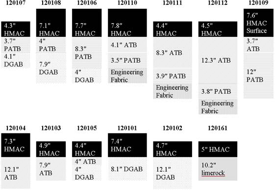
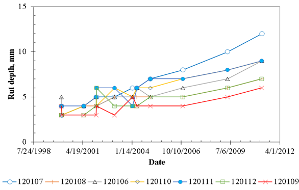
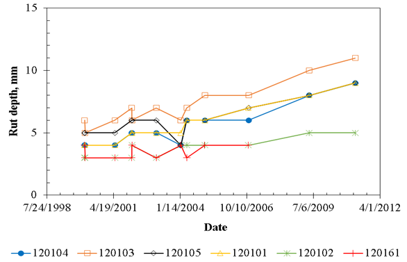
Figure 5 shows the pavement structure in the Florida SPS-1 test sections in the same order that they exist onsite. Figure 6 and figure 7 show the trend in the average section rutting values measured on Florida SPS-1 test sections from 2000 to 2011. As it can be seen, despite the increasing trend in rutting values with time, the trends for different test sections are not parallel to each other, and they cross at several points. This indicates the inherent variability in the involved parameters and the measurement methods. Also, the averaging of rutting values from different locations on each test section obscures the real trends.
Source: FHWA.
HMAC = hot-mix asphalt concrete; DGAB = dense-graded aggregate base.
Figure 5. Illustration. Pavement structure in Florida SPS-1 test sections.
Source: FHWA.
Figure 6. Chart. Average rutting measurements on SPS-1 test sections 120107 to 120109.
Source: FHWA.
Figure 7. Chart. Average rutting measurements on SPS-1 test sections 120104 to 120161.
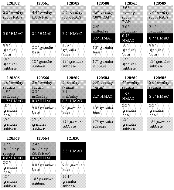
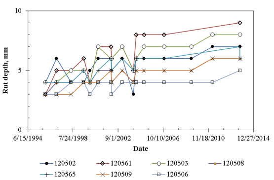
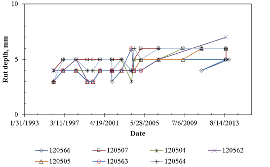
Figure 8 shows the pavement structure in the Florida SPS-5 test sections in the same order that they exist on the site. Figure 9 and figure 10 show the trend in the average section rutting values measured on Florida SPS-5 test sections from 1995 to 2013.
Source: FHWA.
Figure 8. Illustration. Pavement structure in Florida SPS-5 test sections.
Source: FHWA.
Figure 9. Chart. Average rutting measurements on SPS-5 test sections.
Source: FHWA.
Figure 10. Chart. Average rutting measurements on SPS-5 test sections.
FDOT has an APT facility with a heavy vehicle simulator (HVS). FDOT has used this facility for conducting several AC pavement experiments, of which two were selected in this project to provide information for the rutting calibration process.
Dominant Aggregate Size Range Gradation Model Experiment
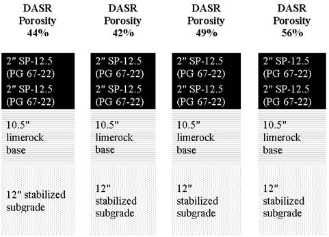
FDOT established an accelerated pavement experiment to test various aggregate gradations to resist rutting. The approach taken by FDOT is known as the dominant aggregate size range (DASR) gradation model. Four sections were built to be tested under the HVS. Test sections were trafficked at 50 ºC using a 455-mm wide-base single tire inflated to 390 kPa and loaded to 40 kN.(53)
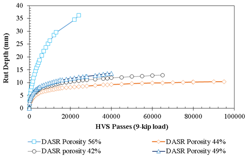
Each test section consisted of two layers of HMA of 2 inches. Those layers were placed over a 20.5-inch limerock base and a 12-inch limerock stabilized subgrade. The DASR porosity ranged from 42 to 56 percent, and mixes with lower DASR porosity exhibited less rutting. Figure 11 presents a schematic of the pavement structure in the four test sections, and figure 12 shows the rutting measurements.
Source: FHWA.
SP-12.5 = Superpave with nominal maximum aggregate size of 12.5 inches.
Figure 11. Illustration. FDOT DASR project sections.(54)
Source: FHWA.
Figure 12. Chart. Rutting for the four sections tested under FDOT DASR project.
Asphalt Rubber Binder Experiment
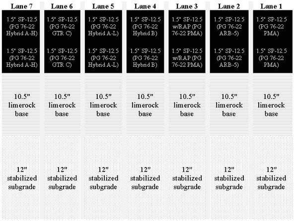
FDOT built a set of seven APT sections as a part of a study to compare HMA mixtures constructed using a polymer-modified asphalt (PMA) and an asphalt rubber binder (ARB). The objective of this study was to find a way to make ARB handle and perform similarly to PG 76-22, Florida’s “gold standard” binder. The experiment included three PMA sections and four ARB sections. Testing lanes were milled and resurfaced, approximately 1 inch of existing asphalt remained in place after milling, and then each lane was resurfaced with two 1.5-inch layers of a 12.5-inch nominal maximum aggregate size fine-graded Superpave mixture. The asphalt mixtures of each lane were the same except for the binder type.(54)
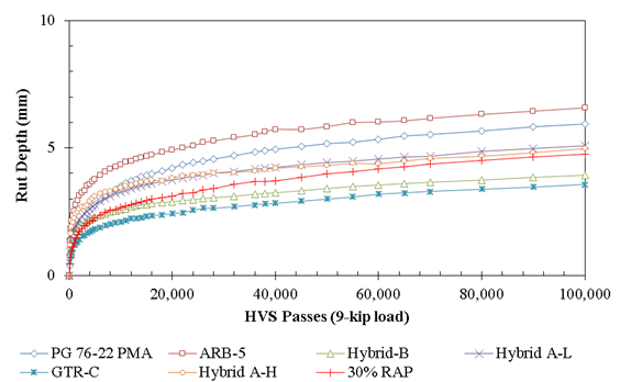
Figure 13 presents a schematic of the pavement structure in the four test sections, and figure 14 shows the rutting measurements.
Accelerated loading was performed using FDOT’s HVS with a super single tire loaded to 9 kip and inflated to 110 psi. A wheel wander of 4 inches was used and the test temperature maintained at 50 ºC. All the mixtures showed good rutting performance. All mixtures with a PG 76-22 (ARB) exhibited slightly better rutting resistance than the control mix.
Source: FHWA.
GTR = ground tire rubber.
Figure 13. Illustration. FDOT ARB project sections.
Source: FHWA.
Figure 14. Chart. Rutting for the seven sections tested under FDOT ARB project.