U.S. Department of Transportation
Federal Highway Administration
1200 New Jersey Avenue, SE
Washington, DC 20590
202-366-4000
Federal Highway Administration Research and Technology
Coordinating, Developing, and Delivering Highway Transportation Innovations
| REPORT |
| This report is an archived publication and may contain dated technical, contact, and link information |
|
| Publication Number: FHWA-HRT-17-104 Date: June 2018 |
Publication Number: FHWA-HRT-17-104 Date: June 2018 |
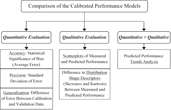
A comprehensive framework was devised for comparison of the multi-objective calibration results to the AASHTO recommended single-objective calibration. This comparison framework is based on quantitative and qualitative evaluation of the calibrated models.(63) Figure 17 shows the different steps within the comparison framework.
The measured rutting databases for both LTPP and APT were randomly divided into 80 percent for calibration and 20 percent for validation. Following the calibration of the models using the calibration data, the calibrated prediction models were tested using the validation dataset.
Source: FHWA.
Figure 17. Flowchart. Framework for comparison of the calibrated performance models.
For quantitative evaluation, accuracy, precision, and generalization capability of the models are assessed using the calibration and validation datasets. To evaluate the accuracy of the multi-objective approach compared to the conventional single-objective calibration, statistical significance testing is required to determine whether the bias between measured and predicted performance values is statistically significant before and after each calibration process.
The bias (average error) is an estimate of the model accuracy, and the STE represents the precision of the performance model. According to the AASHTO recommended calibration guidelines, the STE of the calibrated model is compared to the STE from the national global calibration to determine its significance.
Once the models are calibrated, they are validated on a validation dataset to check for the reasonableness of performance predictions. This step also provides a measure of the generalization capability (repeatability) of the calibrated models. The model that generalizes better will be the model that matches measured pavement performance equally well on both the validation and the calibration datasets.
For qualitative evaluation of the calibrated models, scatterplots of measured versus predicted performance on the calibration and validation datasets were used. Another qualitative assessment could be a sensitivity analysis of the calibrated models to the changes in input variables, which is a substantial task and beyond the scope of the current project. The reasonableness of this model behavior can be compared between the single-objective and multi-objective calibration methods. An additional qualitative evaluation was conducted by comparing the shape of the distribution of measured versus predicted pavement performance. Statistical distribution shape descriptors such as nonparametric skewness and kurtosis can be used for this purpose.
Examining the predicted rate of change in performance indices compared to measured deterioration trends, a combination of quantitative and qualitative evaluations was implemented to compare different calibrated models.
This comparison of the multi-objective approach to the conventional single-objective method is demonstrated in calibrating rutting models for new AC pavements using LTPP SPS-1 Florida site data, new AC pavements using FDOT APT data, and overlaid AC pavements using LTPP SPS-5 Florida site data.
A single-objective calibration according to the AASHTO guidelines was conducted, the results of which serve as a comparison baseline. The AASHTO recommended approach includes an 11-step procedure for “verification,” “calibration,” and “validation” of the MEPDG models for local conditions. The verification involves an examination of accuracy and precision of the global (nationally calibrated) model on the local dataset.
Table 26 and table 27 list the important statistics regarding this verification of the rutting models for new pavements using Florida SPS-1 site data and overlaid pavements using Florida SPS-5 site data, respectively. As expected, the results show a significant positive bias and a high standard deviation of error because the global model was calibrated based on all LTPP data from across North America. The next steps will demonstrate the AASHTO recommended procedure for “eliminating” the bias and potentially reducing the STE.
Table 26. “Verification” of the global rutting model for new pavements on Florida SPS-1.
| Statistic | Calibration Data | Validation Data | Combined Data |
|---|---|---|---|
| Data records | 128 | 26 | 154 |
| SSE | 11,135.13 mm2 (17.26 inch2) |
2,396.75 mm2 (3.72 inch2) |
13,531.88 mm2 (20.97 inch2) |
| RMSE | 9.33 mm (0.367 inch) | 9.60 mm (0.379 inch) | 9.37 mm (0.370 inch) |
| Bias | +8.05 mm (0.317 inch) | +8.34 mm (0.328 inch) | +8.10 mm (0.319 inch) |
| p value (paired t-test) for bias | 5.11E – 39 < 0.05; significant bias | 1.28E – 08 < 0.05; significant bias | 5.51E – 47 < 0.05; significant bias |
| STE | 4.73 mm (0.186 inch) | 4.85 mm (0.191 inch) | 4.73 mm (0.186 inch) |
| Generalization capability | N/A | N/A | 96.4% |
| R2 (goodness of fit) | 0.0391 | 0.123 | 0.0487 |
| RMSE = root-mean-squared error; generalization capability = 100 – normalized difference in bias between the calibration and validation datasets. N/A = not applicable. | |||
Table 27. “Verification” of the global rutting model for overlaid pavements on Florida SPS-5.
| Statistic | Calibration Data | Validation Data | Combined Data |
|---|---|---|---|
| Data records | 189 | 39 | 228 |
| SSE | 62,207.04 mm2 (96.42 inch2) |
11,607.67 mm2 (17.99 inch2) |
73,814.71 mm2 (114.41 inch2) |
| RMSE | 18.14 mm (0.714 inch) | 17.25 mm (0.680 inch) | 17.99 mm (0.709 inch) |
| Bias | +16.39 mm (0.645 inch) | +15.71 mm (0.618 inch) | +16.27 mm (0.640 inch) |
| p value (paired t-test) for bias | 7.40E – 71 < 0.05; significant bias | 1.18E– 15 < 0.05; significant bias | 9.78E– 86 < 0.05; significant bias |
| STE | 7.80 mm (0.311 inch) | 7.22 mm (0.284 inch) | 7.70 mm (0.304 inch) |
| Generalization capability | N/A | N/A | 95.85% |
| R2 (goodness of fit) | 0.0609 | 0.0018 | 0.0504 |
| N/A = not applicable; RMSE = root-mean-squared error. | |||
At the seventh step of the 11-step AASHTO recommended calibration procedure, the significance of the bias (the average difference between predicted and measured performance) is tested. If there is a significant bias in prediction of pavement performance measures, the first round of calibration is conducted at the eighth step to eliminate bias. During this step, the SSE is minimized by adjusting the βr1, βGB, and βSG calibration factors.
At the ninth step, the STE (standard deviation of error among the calibration dataset) is evaluated by comparing it to the STE from the national global calibration, which was about 0.1 inch. If there is a significant STE, the second round of calibration at the tenth step tries to reduce the STE by adjusting the βr2 and βr3 calibration factors. A final validation step checks for the reasonableness of performance predictions on the validation dataset that has not been used for model calibration.
Global heuristic optimization methods such as EAs could possibly identify a more optimum set of calibration coefficients compared to the local exhaustive search methods. That is why in this project GA was used for single-objective optimization in calibrating rutting models for new AC pavements using the LTPP SPS-1 Florida site data and overlaid AC pavements using the LTPP SPS-5 Florida site data.
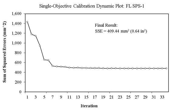
Figure 18 shows a dynamic plot of SSE as the optimization iterations pass by for single-objective calibration on Florida SPS-1 data. The optimization is stopped when the SSE for the best member of the population does not change more than 1 mm2 for at least 10 consecutive generations (in this case, after 34 iterations).
Source: FHWA.
Figure 18. Chart. Dynamic plot of SSE in single-objective optimization on Florida SPS-1 data.
Table 28 lists the important statistics regarding these single-objective calibration results of rutting models for new pavements on Florida SPS-1. The final results of the single-objective minimization of SSE demonstrate a p value (0.096) greater than 0.05 for a paired t-test of measured versus predicted total rut depth on calibration data. Therefore, there is not enough evidence to reject the null hypothesis of the bias being insignificant. It seems that the continuation of this optimization process will not significantly improve the results (figure 18). On the other hand, the p value is much higher (0.47) for the validation dataset, and therefore the bias seems to be even less significant on the validation dataset, which was not used for model calibration. The negative bias indicates that the calibrated model underpredicts rut depth values on average by 0.25 mm, which is insignificant compared to the accuracy of manual rut depth measurements that is 1 mm in the LTPP program.
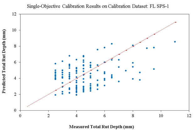
There seems to be a lack of precision of the calibrated model demonstrated by the high amount of scatter in figure 19. However, since the overall STE is lower than the national global calibration results (0.068 inch < 0.129 inch), according to AASHTO calibration guidelines, there is no need for the second round of optimization to reduce STE. Therefore, the following are the selected calibration factors:
βr1 = 0.522, βr2 = 1.0, βr3 = 1.0, βGB= 0.011, and βSG = 0.171.
Table 28. Single-objective calibration results of rutting models for new pavements on Florida SPS-1.
| Statistic | Calibration Data | Validation Data | Combined Data |
|---|---|---|---|
| Data records | 128 | 26 | 154 |
| SSE | 409.44 mm2 (0.64 inch2) | 59.70 mm2 (0.09 inch2) | 469.14 mm2 (0.73 inch2) |
| RMSE | 1.79 mm (0.071 inch) | 1.52 mm (0.060 inch) | 1.75 mm (0.069 inch) |
| Bias | –0.26 mm (–0.010 inch) | –0.20 mm (–0.008 inch) | –0.25 mm (–0.010 inch) |
| p value (paired t-test) for bias | 0.096 > 0.05; insignificant bias | 0.47 > 0.05; insignificant bias | 0.072 > 0.05; insignificant bias |
| STE | 1.78 mm (0.070 inch) | 1.53 mm (0.060 inch) | 1.73 mm (0.068 inch) |
| Generalization capability | N/A | N/A | 70% |
| R2 (goodness of fit) | 0.1519 | 0.2553 | 0.165 |
| N/A = not applicable; RMSE = root-mean-squared error. | |||
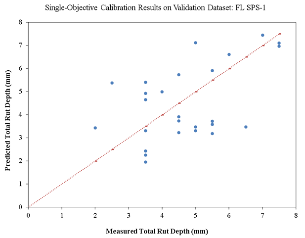
Figure 19 and figure 20 show scatterplots of the measured versus predicted total rut depth on calibration (128 records) and validation (26 records) datasets, respectively, for Florida SPS-1. The measured rut depth data are discrete values at every 1 mm (the plots show 0.5 mm because the rut depth values are averaged between the left and right wheelpaths), while the predicted rut depth data are continuous values. Even though the bias and the STE are relatively low on both the calibration and validation datasets, there is a significant amount of scatter in these plots, and the goodness-of-fit indicator (R2) is poor. This scatter could perhaps be due to two reasons. First and foremost, the calibrated model does not exhibit adequate precision. This could be tracked back to the lack of precision of the global model. Second, there is a high degree of variation (perhaps due to construction quality and environmental variability) in measured rut depths along each pavement section (and between the two wheelpaths) at each distress survey, while the model can only produce one value (for 50 percent reliability) for each pavement section at each specified time. This could add to the scatter observed in these plots.
Source: FHWA.
Figure 19. Scatterplot. Measured versus predicted single-objective calibration results of rutting models for new pavements on calibration dataset for Florida SPS-1.
Source: FHWA.
Figure 20. Scatterplot. Measured versus predicted single-objective calibration results of rutting models for new pavements on validation dataset for Florida SPS-1.
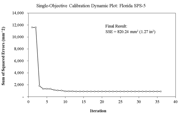
Figure 21 shows a dynamic plot of SSE as the optimization iterations pass by for single-objective calibration on Florida SPS-5 data. The optimization is stopped when the SSE for the best member of the population does not change more than 1 mm2 for at least 10 consecutive generations (in this case, after 36 iterations).
Source: FHWA.
Figure 21. Chart. Dynamic plot of SSE in single-objective optimization on Florida SPS-5 data.
Table 29 lists the important statistics regarding these single-objective calibration results of rutting models for overlaid pavements on Florida SPS-5. The final results of the single-objective minimization of SSE demonstrate a low p value (0.0005) for a paired t-test of measured versus predicted total rut depth on calibration data. Therefore, the null hypothesis of the bias being insignificant has been rejected. However, it seems that the continuation of this optimization process will not significantly improve the results (figure 21). The p value is higher (0.013) for the validation dataset, but the bias is still significant on the validation dataset as well.
Table 29. Single-objective calibration results of rutting models for overlaid pavements on Florida SPS-5.
| Statistic | Calibration Data | Validation Data | Combined Data |
|---|---|---|---|
| Data records | 189 | 39 | 228 |
| SSE | 820.24 mm2 (1.27 inch2) | 128.37 mm2 (0.20 inch2) | 948.61 mm2 (1.47 inch2) |
| RMSE | 2.08 mm (0.082 inch) | 1.81 mm (0.071 inch) | 2.04 mm (0.080 inch) |
| Bias | –0.53 mm (–0.021 inch) | –0.72 mm (–0.028 inch) | –0.56 mm (–0.022 inch) |
| p value (paired t-test) for bias | 0.0005 < 0.05; significant bias | 0.013 < 0.05; significant bias | 3.18E-05 < 0.05; significant bias |
| STE | 2.02 mm (0.080 inch) | 1.69 mm (0.066 inch) | 1.97 mm (0.078 inch) |
| Generalization capability | N/A | N/A | 64.15% |
| R2 (goodness of fit) | 0.1196 | 0.0213 | 0.1073 |
| N/A = not applicable; RMSE = root-mean-squared error. | |||
Since the overall STE is lower than the national global calibration results (0.078 inch < 0.129 inch), according to AASHTO calibration guidelines, there is no need for the second round of optimization to reduce STE. Therefore, the following are the selected calibration factors:
βr1 = 0.5004, βr2 = 1.0, βr3 = 1.0, βGB= 0.0738, and βSG = 0.1554.
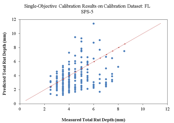
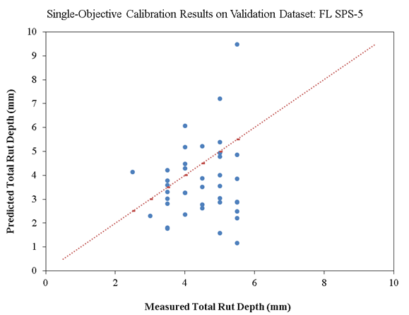
Figure 22 and figure 23 show scatterplots of the measured versus predicted total rut depth on calibration (189 records) and validation (39 records) datasets, respectively, for Florida SPS-5. Similar to the results on SPS-1 data, there is a significant amount of scatter in these plots, and the goodness-of-fit indicator (R2) is poor. The negative bias indicates that the calibrated model underpredicts rut depth values on average by 0.56 mm. While this bias is statistically significant, it is low compared to the accuracy of manual rut depth measurements, which is 1 mm in the LTPP program.
Source: FHWA.
Figure 22. Scatterplot. Measured versus predicted single-objective calibration results of rutting models for overlaid pavements on calibration dataset for Florida SPS-5.
Source: FHWA.
Figure 23. Scatterplot. Measured versus predicted single-objective calibration results of rutting models for overlaid pavements on validation dataset for Florida SPS-5.
As discussed in chapter 4, several scenarios can be devised for multi-objective formulation of calibration, all of which could overcome cognitive challenges and add to our knowledge of this problem. The following sections demonstrate the results of the two considered scenarios—the first for simultaneous utilization of multiple statistical data in the calibration process, and the second for objective incorporation of data from multiple disparate sources. Note that in the multi-objective calibration approaches, unlike the single-objective calibration, all of the involved calibration factors are evolved to determine the suitable factors.
The general goal of any multi-objective optimization is to identify the Pareto-optimal tradeoffs between multiple objectives. A Pareto-optimal tradeoff identifies the best compensation among the multiple conflicting objectives. The solutions presented on the Pareto-optimal front are nondominated solutions. A solution X1 is called dominated if, and only if, another feasible solution X2 performs better than X1 in terms of at least one objective and as well as X1 in terms of others. A set of nondominated solutions is called the nondominated or Pareto-optimal front. This nondominated solution set might contain information that advances knowledge of the problem at hand.
The final solution can be selected from the set using engineering judgment and/or other qualitative criteria. Statistical distribution shape descriptors (skewness and kurtosis) can be used in conjunction with engineering judgment to better match the distribution of measured and calculated rutting data on LTPP test sections. Difference in nonparametric skew (as calculated using equation 46) between the distributions of measured and calculated rutting values could be one of the criteria used to select the final solution among the nondominated pool of solutions. Skewness quantifies how symmetrical the distribution is.
![]() (46)
(46)
Where:
NPS = non-parametric skewness.
μ = mean.
ν = median.
σ = standard deviation.
Another criterion is the difference in kurtosis (as calculated using equation 47) between the distributions of measured and calculated rutting values. Kurtosis quantifies whether the shape of the data distribution matches the Gaussian distribution. A flatter distribution has a negative kurtosis, and a distribution more peaked than a Gaussian distribution has a positive kurtosis.
![]() (47)
(47)
In the first alternative scenario, mean and standard deviation of prediction error were simultaneously minimized to reduce the bias and STE (increase model accuracy and precision) at the same time. In this manner, the information from a single calibration run was fully implemented, and an additional round of computationally intensive calibration was avoided.
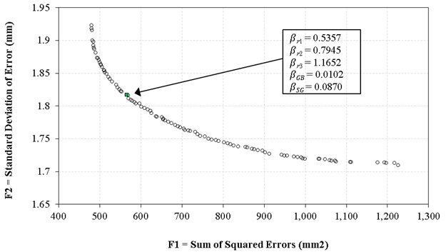
Figure 24 presents the final Pareto-optimal front showing the nondominated solutions in terms of SSE and STE for the SPS-1 data. As explained in chapter 4, it cannot be proven whether the selected objective functions are in conflict. In other words, decreasing SSE might not necessarily decrease STE. As shown in this graph, the results of this specific optimization indicate that decreasing one objective might result in increasing the other. Since the two objectives of minimizing bias (increasing accuracy) and minimizing STE (increasing precision) seem to be conflicting objectives in this case, the application of a multi-objective optimization algorithm is justified. This means that a final calibrated model that exhibits higher accuracy might not necessarily have higher precision as well. In this specific case, the difference in STE is not significant among the different solutions.
Source: FHWA.
Figure 24. Scatterplot. The final nondominated solution set for two-objective calibration of rutting models for new pavements on Florida LTPP SPS-1 data.
All the solutions on this nondominated front are valid solutions in terms of the mathematical optimization problem at hand. This is because no solution is better than another solution in terms of all objective functions. A solution might perform better than another in terms of one objective function (e.g., higher accuracy), but it will be performing worse in terms of the other objective function (e.g., lower precision). However, qualitative criteria and engineering judgment could be practiced when selecting the most reasonable solution from this front.
Table 30 shows two of the candidate solutions on the final nondominated front for SPS-1 data (figure 24). These solutions have the minimum difference in skewness and kurtosis between the predicted and measured rutting values. Based on these results, the solution with minimum skewness difference seems to be the suitable solution, as its difference in kurtosis is not much higher than the solution with minimum kurtosis difference:
βr1 = 0.54, βr2 = 0.79, βr3 = 1.16, βGB= 0.01, and βSG = 0.09.
Table 30. Candidate solutions from the two-objective nondominated front for SPS-1, with minimum difference in skewness and kurtosis between predicted and measured distributions.
| Candidate Solutions | βr1 | βr2 | βr3 | βGB | βSG | SSE (mm2) | STE (mm) | Skewness Difference (%) | Kurtosis Difference (%) |
|---|---|---|---|---|---|---|---|---|---|
| Minimum difference in skewness | 0.5357 | 0.7945 | 1.1652 | 0.0102 | 0.0870 | 494.19 | 1.66 | 43.27 | 34.48 |
| Minimum difference in kurtosis | 0.5224 | 0.8152 | 1.1548 | 0.0101 | 0.0118 | 617.18 | 1.79 | 55.40 | 33.18 |
It should be noted that this solution (highlighted in figure 24) also provides a more reasonable (farther from zero) calibration factor for the subgrade rutting, compared to the single-objective calibration results. The calibration factor for rutting in the base layer seems insignificant, but all the solutions on the nondominated front shared this issue. Since trench data were not available for this study, the models could not be calibrated accurately for the rutting in unbound layers, as they are often overwhelmed by bound layers with higher stiffness.
The final results in table 31 demonstrate a low p value for a paired t-test of measured versus predicted total rut depth on the calibration dataset. Therefore, the null hypothesis of the bias being insignificant has been rejected. The p value is higher for the validation dataset (0.001), but the bias is still significant on the validation dataset as well. The negative bias indicates that the calibrated model underpredicts rut depth values on average by 1.05 mm, which is at the same accuracy of manual rut depth measurements that is 1 mm in the LTPP program.
Table 31. Two-objective calibration results of rutting models for new pavements on Florida SPS-1.
| Statistic | Calibration Data | Validation Data | Combined Data |
|---|---|---|---|
| Data records | 128 | 26 | 154 |
| SSE | 494.19 mm2 (0.77 inch2) | 72.41 mm2 (0.11 inch2) | 566.60 mm2 |(0.88 inch2) |
| RMSE | 1.96 mm (0.077 inch) | 1.67 mm (0.066 inch) | 1.92 mm (0.076 inch) |
| Bias | –1.06 mm (–0.042 inch) | –1.01 mm (–0.040 inch) | –1.05 mm (–0.041 inch) |
| p value (paired t-test) for bias | 4.56E-11 < 0.05; significant bias | 0.001 < 0.05; significant bias | 1.68E-13 < 0.05; significant bias |
| STE | 1.66 mm (0.065 inch) | 1.36 mm (0.054 inch) | 1.61 mm (0.063 inch) |
| Generalization capability | N/A | N/A | 95.28% |
| R2 (goodness of fit) | 0.1778 | 0.3067 | 0.194 |
| N/A = not applicable; RMSE = root-mean-squared error. | |||
In comparison to the single-objective calibration results, the two-objective calibration has resulted in lower accuracy (a higher bias), but higher precision (a lower STE), of the final model on both the calibration and validation datasets. This is because the standard deviation of error was also minimized simultaneously with the SSE. In addition to an increased precision, the other improvement is the generalization capability of the calibrated model. The model that was calibrated using two-objective optimization had more similar bias values on calibration and validation data, compared to the single-objective results.
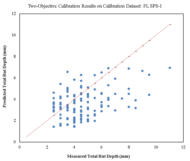
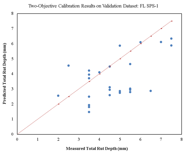
Figure 25 and figure 26 show scatterplots of the measured versus predicted total rut depth on calibration (128 records) and validation (26 records) datasets, respectively, for Florida SPS-1. Similar to the single-objective calibration results, there is a significant amount of scatter in these plots, and the goodness-of-fit indicator (R2) is poor. As explained before, this scatter indicates the lack of precision of the rutting model. However, the overall STE is lower than the national global calibration results (0.063 inch < 0.129 inch).
Overall, it seems that the two-objective optimization has increased the precision and generalization capability of the final calibrated model at the cost of decreasing accuracy. Since the changes in the results are not significant, conducting scenario 1 of the multi-objective optimization might not be worth the computational cost.
Source: FHWA.
Figure 25. Scatterplot. Measured versus predicted two-objective calibration results of rutting models for new pavements on calibration dataset for Florida SPS-1.
Source: FHWA.
Figure 26. Scatterplot. Measured versus predicted two-objective calibration results of rutting models for new pavements on validation dataset for Florida SPS-1.
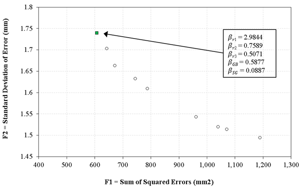
From the two-objective Pareto-optimal front on SPS-1 (figure 24), it seems that using an epsilon parameter (MOEA precision factor) of 0.1 was too conservative and has produced too many solutions with similar objective function values. A higher epsilon value (equal to 1.0 instead of 0.1) was used for the two-objective calibration on SPS-5 data, and that has increased the speed and efficiency of the multi-objective optimization drastically (by about 70 percent). Figure 27 shows the final Pareto-optimal front showing the nondominated solutions in terms of SSE and STE for the SPS-5 data.
Again, the skewness and kurtosis of the predicted rutting distribution with every solution on the nondominated front were calculated and compared to the measured values (table 32). From these calculations, it is evident that one of the solutions on the final front produces rutting predictions that have the lowest difference in distribution skewness and kurtosis from the distribution of measured rut depth values. However, there is another similar solution (in bold font) that has resulted in the most reasonable calibration factor for the subgrade rutting. The final selected solution is also highlighted in figure 27.
Source: FHWA.
Figure 27. Scatterplot. The final nondominated solution set for two-objective calibration of rutting models for overlaid pavements on Florida LTPP SPS-5 data.
Table 32. Solutions from the two-objective nondominated front for SPS-5, with difference in skewness and kurtosis between predicted and measured data distributions.
| Candidate Solutions | βr1 | βr2 | βr3 | βGB | βSG | SSE (mm2) | STE (mm) | Skewness Difference (%) | Kurtosis Difference (%) |
|---|---|---|---|---|---|---|---|---|---|
| Other viable solution | 1.8778 | 0.7588 | 0.5071 | 0.4438 | 0.0226 | 1,188.72 | 1.49 | 52.33 | 19.48 |
| Other viable solution | 2.1152 | 0.9602 | 0.5071 | 0.4405 | 0.0246 | 1,070.47 | 1.51 | 58.65 | 29.54 |
| Other viable solution | 2.1152 | 0.9602 | 0.5071 | 0.5877 | 0.0246 | 744.75 | 1.63 | 61.78 | 25.72 |
| Other viable solution | 2.1185 | 0.9939 | 0.5069 | 0.4370 | 0.0256 | 1,039.45 | 1.52 | 51.96 | 33.24 |
| Other viable solution | 2.1185 | 0.9939 | 0.5069 | 0.4746 | 0.0225 | 961.70 | 1.54 | 59.60 | 31.58 |
| Minimum skewness and kurtosis difference | 2.9712 | 0.7589 | 0.5071 | 0.5877 | 0.0253 | 787.72 | 1.61 | 51.89 | 19.28 |
| Other viable solution | 2.9838 | 0.7589 | 0.5071 | 0.5877 | 0.0540 | 671.14 | 1.66 | 56.40 | 22.83 |
| Other viable solution | 2.9844 | 0.7589 | 0.5071 | 0.5877 | 0.0887 | 541.80 | 1.64 | 53.49 | 25.64 |
| Other viable solution | 2.9844 | 0.9599 | 0.5071 | 0.5877 | 0.0500 | 643.39 | 1.70 | 56.25 | 31.35 |
The final selected solution seems to have reasonable calibration factors for base and subgrade rutting: βr1 = 2.98, βr2 = 0.76, βr3 = 0.51, βGB= 0.59, and βSG = 0.09. Table 33 shows the prediction results of this final solution on SPS-5 calibration and validation datasets. While the low bias value of –0.44 mm is much less than the LTPP measurement precision of 1 mm, the bias is statistically significant on the calibration dataset. However, the bias is statistically insignificant on the validation dataset that was not used in the calibration process.
Table 33. Two-objective calibration results of rutting models for overlaid pavements on Florida SPS-5.
| Statistic | Calibration Data | Validation Data | Combined Data |
|---|---|---|---|
| Data records | 189 | 39 | 228 |
| SSE | 541.80 mm2 (0.84 inch2) | 91.65 mm2 (0.14 inch2) | 633.45 mm2 (0.98 inch2) |
| RMSE | 1.69 mm (0.066 inch) | 1.53 mm (0.060 inch) | 1.67mm (0.066 inch) |
| Bias | –0.44 mm (–0.017 inch) | –0.47 mm (–0.018 inch) | –0.45 mm (–0.018 inch) |
| p value (paired t-test) for bias | 0.0003 < 0.05; significant bias | 0.051 > 0.05; insignificant bias | 4.16E-05 < 0.05; significant bias |
| STE | 1.64 mm (0.065 inch) | 1.48 mm (0.058 inch) | 1.61 mm (0.063 inch) |
| Generalization capability | N/A | N/A | 93.18% |
| R2 (goodness of fit) | 0.0427 | 0.0013 | 0.0348 |
| N/A = not applicable; RMSE = root-mean-squared error. | |||
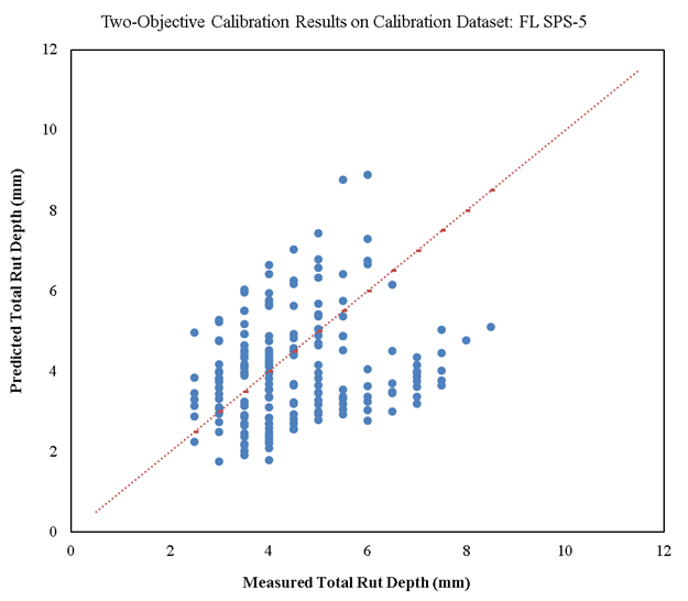
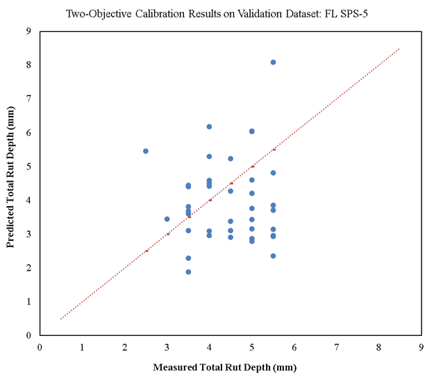
Figure 28 and figure 29 show scatterplots of the measured versus predicted total rut depth on calibration (189 records) and validation (39 records) datasets, respectively, for Florida SPS-5. Similar to the single-objective calibration, there is significant scatter in these plots. However, the standard deviation of error is lower for the model that was calibrated using the two-objective approach compared to the single-objective approach. The overall standard deviation of error is much lower than the STE from the national global calibration (0.063 < 0.129).
Compared to the single-objective calibration, the rutting model for overlaid pavements (SPS-5) that was calibrated using the two-objective approach shows both a higher accuracy and higher precision. In addition, the two-objective calibration has resulted in a model with much greater generalization capability.
Source: FHWA.
Figure 28. Scatterplot. Measured versus predicted two-objective calibration results of rutting models for overlaid pavements on calibration dataset for Florida SPS-5.
Source: FHWA.
Figure 29. Scatterplot. Measured versus predicted two-objective calibration results of rutting models for overlaid pavements on validation dataset for Florida SPS-5.
In the second scenario, the SSE and STE in predicting permanent deformation of pavements within different performance data sources were used as separate objective functions to be minimized simultaneously. This four-objective optimization was used in calibrating rutting models for new AC pavements using the LTPP SPS-1 Florida site data and the FDOT APT data at the same time. In this manner, information from pavement performance near the end of its service life can be incorporated in the calibration process. This scenario comprised an objective approach to incorporate different sources of data. This scenario was not applied to overlaid pavements because the available APT data were only for new pavement structures.
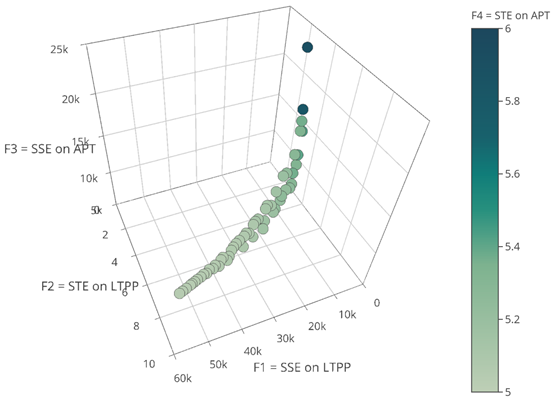
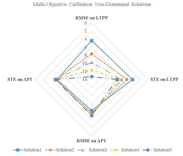
Figure 30 shows the Pareto-optimal front for the four-objective calibration of the rutting models for new pavements using SPS-1 and APT data, simultaneously. In this figure, F1 and F2 are SSE and STE on Florida LTPP SPS-1 data, and F3 and F4 are SSE and STE on FDOT APT data. While F1, F2, and F3 are indicated on the three dimensions, the values for F4 are indicated using a color chart, where lower values are closer to lighter gray. Figure 31 shows another approach to visualizing the final nondominated front for this four-objective optimization. In this figure, root-mean-squared error (RMSE) is shown instead of SSE so that the values of the average error objective functions (F1 and F3) are relatively in the same scale and comparable with standard deviation functions (F2 and F4). Unlike figure 30, where each solution (set of calibration factors) was indicated using a circle, in figure 31, each solution is represented by a line that crosses the objective function axes at different locations.
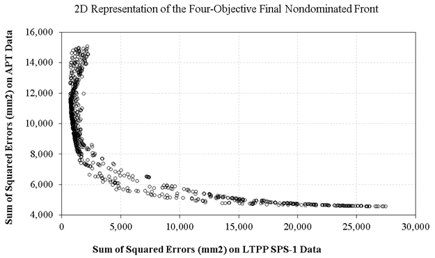
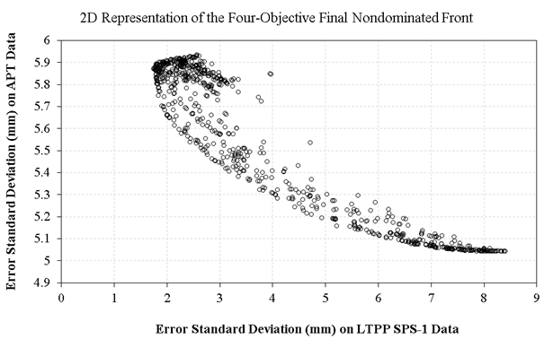
Figure 32 and figure 33 exhibit two-dimensional representations of the final Pareto-optimal front using pairwise comparison of SSE and STE, respectively. Each figure compares the average error or standard deviation of error on SPS-1 data to that on APT data. Note that some solutions on these fronts might seem suboptimal; however, that is because these figures are showing a two-dimensional shadow of the final four-dimensional nondominated front on one plane. Also note that there is a crowd of solutions on these fronts because an epsilon value of 0.1 was used; an epsilon value of 1.0 would result in a more reasonable density of solutions in the final front. Similar to the first multi-objective calibration scenario, these figures show a conflict between the F1 and F3 and F2 and F4 objective functions, which advocates for the application of multi-objective optimization. The advantage of using the multi-objective approach in this case is that solutions closer to the performance measured on SPS-1 sections can be preferred over other solutions closer to the performance observed in APT data. This is because the LTPP sections are actual in-service highway pavements exposed to actual climate and traffic, as opposed to APT sections, which have been exposed to simulated accelerated loading under a constant temperature.
Source: FHWA.
Figure 30. Scatterplot. The final nondominated solution set for four-objective calibration of rutting models for new pavements: F1 and F2 are SSE and STE on Florida LTPP SPS-1 data, and F3 and F4 are SSE and STE on FDOT APT data.
Source: FHWA.
Figure 31. Chart. The final nondominated solution set for four-objective calibration of rutting models for new pavements: RMSE and STE on Florida SPS-1 and FDOT APT data.
Source: FHWA.
Figure 32. Scatterplot. Two-dimensional representation of the final nondominated solution set for four-objective calibration: SSE on Florida LTPP SPS-1 versus SSE on FDOT APT data.
Source: FHWA.
Figure 33. Scatterplot. Two-dimensional representation of the final nondominated solution set for four-objective calibration: STE on Florida LTPP SPS-1 versus STE on FDOT APT data.
Table 34 shows some viable candidate solutions from the final nondominated front. The solution that has the minimum difference in kurtosis between the predicted and measured SPS-1 data is exhibiting a high difference in skewness. Therefore, other candidates with a better balance were sought. Some solutions show a very low value for the calibration factors for either base or subgrade, and those solutions were avoided. Therefore, it seems that the solution with the minimum difference in kurtosis is the best candidate, as it exhibits reasonable calibration factors with relatively good quality distribution of predicted values (in addition to being on the final nondominated front of the multi-objective optimization). Note that this solution offers more reasonable calibration factors for base and subgrade layers compared to the solutions on the single-objective and two-objective calibration (where all of the solutions had insignificant values for the calibration coefficient of the base layer):
βr1 = 3.84, βr2 = 0.96, βr3 = 0.56, βGB = 0.14, and βSG = 0.79.
Table 34. Candidate solutions from the four-objective nondominated front with difference in skewness and kurtosis between the predicted and measured data distributions.
| Candidate Solutions | βr1 | βr2 | βr3 | βGB | βSG | On LTPP Data SSE (mm2) |
On LTPP Data STE (mm) |
Skewness Difference (%) | Kurtosis Difference (%) |
|---|---|---|---|---|---|---|---|---|---|
| Minimum difference in kurtosis | 3.8397 | 0.9549 | 0.5625 | 0.1377 | 0.7861 | 539.53 | 2.05 | 105.03 | 29.52 |
| Minimum difference in skewness | 3.8476 | 0.6471 | 0.8332 | 1.4298 | 0.4571 | 1,288.64 | 3.03 | 11.41 | 53.79 |
| Other viable solution | 1.2356 | 0.6223 | 0.7848 | 0.7718 | 0.7178 | 893.73 | 2.64 | 30.82 | 44.60 |
| Other viable solution | 6.2883 | 0.5961 | 0.9930 | 0.0104 | 0.5231 | 736.54 | 2.27 | 139.10 | 35.43 |
| Other viable solution | 1.0952 | 1.4996 | 0.5051 | 1.3954 | 0.0140 | 2,354.96 | 3.99 | 58.50 | 52.62 |
| Other viable solution | 1.0952 | 1.4559 | 0.5016 | 0.0560 | 0.0189 | 823.28 | 2.28 | 151.96 | 41.42 |
| Other viable solution | 0.9257 | 0.8089 | 1.0421 | 0.0206 | 0.1975 | 1,090.185 | 1.87 | 139.77 | 38.17 |
The final results in table 35 demonstrate a high p value for a paired t-test of measured versus predicted total rut depth on both calibration and validation datasets (0.18 and 0.51, respectively). Therefore, there is not enough evidence to reject the null hypothesis of the bias being insignificant. The negative bias indicates that the calibrated model underpredicts rut depth values on average by 0.28 mm, which is insignificant compared to the accuracy of manual rut depth measurements that is 1 mm in the LTPP program.
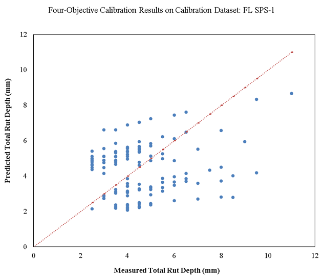
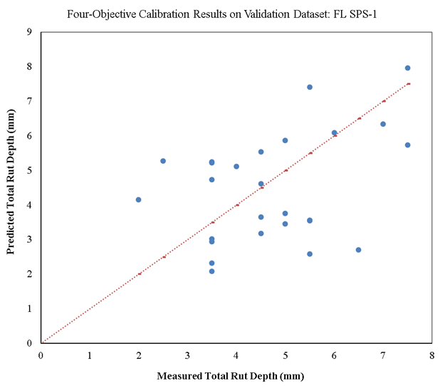
Based on the final selected solution, figure 34 and figure 35 show the measured versus predicted total rut depth on Florida SPS-1 calibration and validation datasets, respectively. Similar to the single-objective and two-objective calibration results, there is a significant amount of scatter in these plots, and the goodness-of-fit indicator (R2) is poor. As explained before, this scatter indicates the lack of precision of the rutting model. However, the overall STE is lower than the national global calibration results (0.078 inch < 0.129 inch).
Table 35. Four-objective calibration results of rutting models for new pavements on Florida SPS-1 data.
| Statistic | Calibration Data | Validation Data | Combined Data |
|---|---|---|---|
| Data records | 128 | 26 | 154 |
| SSE | 539.53 mm2 (0.84 inch2) | 71.13 mm2 (0.11 inch2) | 610.66 mm2 (0.95 inch2) |
| RMSE | 2.05 mm (0.081 inch) | 1.65 mm (0.065 inch) | 1.99 mm (0.078 inch) |
| Bias | –0.24 mm (–0.009 inch) | –0.24 mm (–0.009 inch) | –0.24 mm (–0.009 inch) |
| p value (paired t-test) for bias | 0.18 > 0.05; insignificant bias | 0.51 > 0.05; insignificant bias | 0.125 > 0.05; insignificant bias |
| STE | 2.05 mm (0.081 inch) | 1.67 mm (0.066 inch) | 1.98 mm (0.078 inch) |
| Generalization capability | N/A | N/A | 100% |
| R2 (goodness of fit) | 0.0263 | 0.1478 | 0.0382 |
| N/A = not applicable. | |||
In comparison to the single-objective calibration results, the four-objective calibration has resulted in increased accuracy (lower bias and even higher p value), but lower precision (a higher STE), of the final model on both the calibration and validation datasets. This is because the four-objective scenario has included APT data in addition to the LTPP data, which are different in nature. The main improvement in the results of four-objective calibration compared to single-objective calibration is the increased generalization capability of the calibrated model. The model that was calibrated using four-objective optimization had more similar bias values on calibration and validation data, compared to the single-objective results.
While the four-objective calibration results are not superior to the single-objective results in terms of precision, the simultaneous minimization of error on both LTPP and APT data has actually resulted in higher accuracy and generalization capability of the calibrated model.
Source: FHWA.
Figure 34. Scatterplot. Measured versus predicted four-objective calibration results of rutting models for new pavements on calibration dataset for Florida SPS-1.
Source: FHWA.
Figure 35. Scatterplot. Measured versus predicted four-objective calibration results of rutting models for new pavements on validation dataset for Florida SPS-1.
To investigate the advantages of the novel calibration approach recommended in this study, the final single-objective and multi-objective calibrated models were compared through a comprehensive framework. This framework (figure 17) includes quantitative measures of accuracy, precision, and generalization capability. A model that has high accuracy and precision might not necessarily have an adequate generalization capability, meaning that it would not be able to reproduce the same accuracy when predicting the performance on other similar test sections. The employed qualitative measures include the goodness of fit and similarity of the distribution shape between measured and predicted performance. The quality of the solutions needs to be also examined in terms of the engineering reasonableness of the selected calibration factors. Finally, a combination of quantitative and qualitative criteria is used by comparing the performance trends prediction. The capability of the final calibrated model in predicting future performance trends is an essential feature for pavement design and therefore a significant indicator of the quality of the developed model.
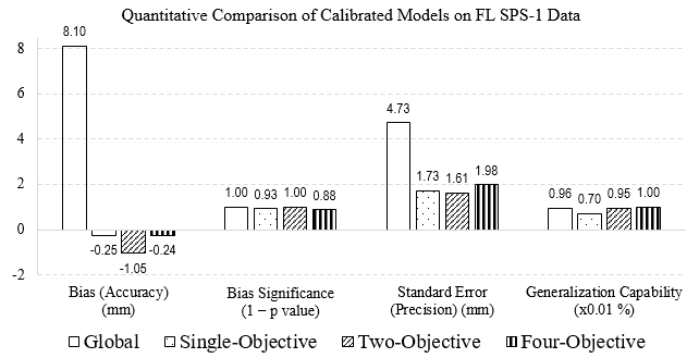
Figure 36 shows a comparison of the quantitative criteria among the single-objective, two-objective, and four-objective calibrated models for rutting in new pavements on combined (calibration and validation) SPS-1 data.
Source: FHWA.
Figure 36. Bar chart. Comparison of the quantitative criteria for the calibrated rutting models on SPS-1.
It is evident in this figure that the incorporation of the APT data in calibration of rutting models on LTPP SPS-1 data has led to a model with the lowest bias (and least significant) and the highest generalization capability. On the other hand, the two-objective minimization of SSE and STE has resulted in the lowest STE (highest precision), but a significant bias (low accuracy).
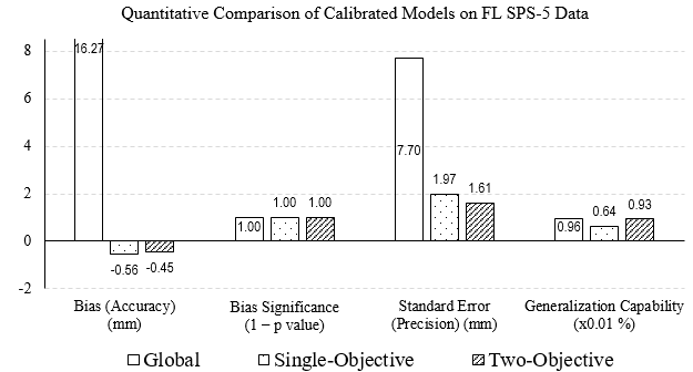
Figure 37 shows a comparison of the quantitative criteria between the single-objective and two-objective calibrated models for rutting in overlaid pavements on combined (calibration and validation) SPS-5 data. There were no APT data available for this calibration of rutting models for overlaid pavements. Unlike the case in calibration on SPS-1 data, the two-objective calibration on SPS-5 data has resulted in both an increase in accuracy (lower bias but still significant), an increase in precision (lower STE), and an increase in generalization capability of the rutting model compared to single-objective calibration.
Source: FHWA.
Figure 37. Bar chart. Comparison of the quantitative criteria for the calibrated rutting models on SPS-5.
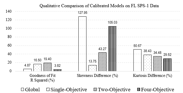
A model that exhibits the best quantitative results might not necessarily show the most desirable qualitative performance. Figure 38 shows a comparison of the qualitative criteria among the single-objective, two-objective, and four-objective calibrated models for rutting in new pavements on combined (calibration and validation) SPS-1 data. The two-objective results show the best goodness of fit, but as explained before, there is a lack of precision of the mechanistic model, and all of the calibration approaches resulted in significant scatter. The single-objective results have the least difference in skewness between the distributions of measured and predicted rutting. The four-objective results show the least difference in kurtosis (flatness) between the distributions of measured and predicted rutting.
Source: FHWA.
Figure 38. Bar chart. Comparison of the qualitative criteria for the calibrated rutting models on SPS-1.
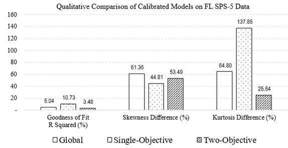
Figure 39 shows a comparison of the qualitative criteria between the single-objective and two-objective calibrated models for rutting in overlaid pavements on combined (calibration and validation) SPS-5 data. The single-objective results show the best goodness of fit and the lowest skewness difference between measured and predicted data. The two-objective results show the least difference in kurtosis (flatness) between the distributions of measured and predicted rutting.
Source: FHWA.
Figure 39. Bar chart. Comparison of the qualitative criteria for the calibrated rutting models on SPS-5.
In all cases, using the multi-objective approach has resulted in predicted rutting distributions that are more similar in flatness to the measured rutting distributions.
Table 36 shows the final selected calibration factors. It is evident that the calibration factors selected for the rutting in base and subgrade layers were insignificant in single-objective calibration. However, the multi-objective calibration has resulted in more reasonable calibration factors for rutting in unbound layers.
Table 36. Final selected calibration factors.
| Model | βr1 | βr2 | βr3 | βGB | βSG |
|---|---|---|---|---|---|
| New pavement (SPS-1) global | 1.0 | 1.0 | 1.0 | 1.0 | 1.0 |
| New pavement (SPS-1) single-objective | 0.522 | 1.0 | 1.0 | 0.011 | 0.171 |
| New pavement (SPS-1) two-objective | 0.536 | 0.795 | 1.165 | 0.010 | 0.087 |
| New pavement (SPS-1) four-objective | 3.840 | 0.955 | 0.563 | 0.138 | 0.786 |
| Overlaid pavement (SPS-5) global | 1.0 | 1.0 | 1.0 | 1.0 | 1.0 |
| Overlaid pavement (SPS-5) single-objective | 0.500 | 1.0 | 1.0 | 0.074 | 0.155 |
| Overlaid pavement (SPS-5) two-objective | 2.984 | 0.759 | 0.507 | 0.588 | 0.089 |
To combine the quantitative and qualitative success metrics of a performance prediction model, the average absolute error (AAE) of the calibrated models in predicting the rate of change in pavement rutting was calculated. The rate of change in rut depth was estimated using measured data and by dividing the change in rutting by the amount of time (months) passed. Only the positive rates were considered in this investigation. Table 37 shows the AAE of the calibrated models in predicting the rate of change in pavement rutting. While the two-objective calibration on SPS-5 data has significantly improved the prediction of rutting deterioration rates compared to single-objective calibration, the multi-objective calibration results on SPS-1 do not exhibit the same quality. This investigation reveals that simply evaluating the bias and STE is not adequate for a comprehensive evaluation of performance prediction models.
Table 37. AAE of calibrated models in predicting the rutting deterioration rates.
| Model | AAE in Predicting the Rate of Change in Rutting (%) |
|---|---|
| New pavement (SPS-1) single-objective | 51.93 |
| New pavement (SPS-1) two-objective | 60.53 |
| New pavement (SPS-1) four-objective | 79.47 |
| Overlaid pavement (SPS-5) single-objective | 100.81 |
| Overlaid pavement (SPS-5) Two-objective | 66.26 |
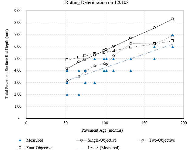
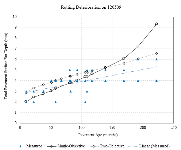
To visualize these deterioration trends, figure 40 and figure 41 demonstrate the measured and predicted rut depth trends on sample test sections of the Florida SPS-1 and SPS-5 sites, respectively. It is evident that on the SPS-1 test section 120108, the two-objective and four-objective calibrations have predicted deterioration trends that are closer to the monitored performance, compared to single-objective calibration results. It should be noted that the predicted rutting data are from the simulated calculations (see chapter 4 for the description of the simulated calculations), and that is why a rutting decrement is observed for the model predictions from the two-objective calibration around the 100th month. The trends on SPS-5 reveal that the two-objective calibration has predicted deterioration trends that better match the measured values, compared to single-objective calibration results.
Source: FHWA.
Figure 40. Chart. Predicted and measured rutting deterioration on FL SPS-1 section 120108.
Source: FHWA.
Figure 41. Chart. Predicted and measured rutting deterioration on FL SPS-5 section 120509.