U.S. Department of Transportation
Federal Highway Administration
1200 New Jersey Avenue, SE
Washington, DC 20590
202-366-4000
Federal Highway Administration Research and Technology
Coordinating, Developing, and Delivering Highway Transportation Innovations
| REPORT |
| This report is an archived publication and may contain dated technical, contact, and link information |
|
| Publication Number: FHWA-HRT-14-064 Date: August 2014 |
Publication Number: FHWA-HRT-14-064 Date: August 2014 |
Physical modeling requires substantial space and time resources that may limit the extent of inquiry. This research also used 3D CFD models to reproduce the complexity of the flows in culverts. CFD allowed for analysis of a more comprehensive set of conditions than was possible in the experimental flume, given the space and budget constraints of the study.
Several CFD modeling software packages are available for simulating flow conditions in a culvert. For this research, CD-adapco's STAR-CCM+ commercial software was used to analyze hydraulic conditions in several culvert configurations. The suitability of CFD modeling for fish passage analysis was assessed by comparing its results with experimental data obtained from the flume modeling.
The first CFD models were of the experimental flume. A 3D multiphase computer-aided design (CAD) model, as shown in figure 15, was created using Pro-ENGINEER. The CAD model consisted of three parts along the flow direction (x-axis): the intake, the barrel, and the diffuser. The culvert model considered in this phase of the study was a symmetrical half section of the culvert pipe having annular corrugations with no embedment.
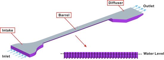
Figure 15. Illustration. 3D CAD model for initial CFD simulations
CFD models are based on a computational mesh. The mesh must capture the boundary layer and preserve the near-wall thickness for the wall function to apply. Because the interface between water and air is an area with steep velocity gradients, mesh refinement volumetric control is used in this study. The resulting meshes are very detailed. For example, a model with a flow depth of 6 inches and an air domain of 3 inches may result in as many as 18 million mesh cells if the basic size is defined as 0.394 inches and the size of refined cells is 0.197 inches. The meshing model and the meshing refinement art are illustrated in figure 16.
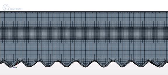
Figure 16. Illustration. Enlarged view of a mesh on the left hand side of the flow direction
A RANS numerical method has been employed in conjunction with a k-epsilon turbulence model and wall function technique for the simulation of complex 3D flow in the culvert. The volume of fluid (VOF) method, which captures the free surface profile through use of the variable known as the volume of fluid, was used in the two-phase (water and air) CFD model. The following physics models were enabled in the computational domain to replicate and simulate the realistic flow conditions: unsteady, liquid, segregated flow, constant density, k-ε turbulence, segregated fluid isothermal, and gravity.
Several strategies for CFD modeling were evaluated. Building a full two-phase (water and air) model of the entire culvert is the most flexible approach but is computationally intensive. One simplifying alternative is to build a single-phase (water only) model neglecting the role of the air layer. A second simplifying alternative is to truncate the model using only a fraction of the entire culvert length and applying a cyclic boundary condition. Both simplifications reduce run times.
Single Versus Two-Phase Modeling
The initial CFD modeling efforts explored representation of culvert flow conditions using the hypothesis of uniform flow in attempting to match conditions in the experimental flume. For uniform flow in a prismatic section, cross-sections exhibit the same velocity distribution throughout the model length. A two-phase (water and air) CFD model was prepared to simulate the change of the water surface within the culvert. A boundary condition is to define the water surface as the interface between the water and air layers. The VOF method was used in the STAR-CCM+ to handle the free water surface.(23)
The two-phase CFD model was created to strictly follow the physical dimensions of the half-section 3-ft diameter CMP culvert without embedment in the experimental flume. The simulations involved three water depths at the 0.71 ft/s flow velocity as described in table 1 for the flume. Specification of the CFD model included description of the flume tilt angle, flap gate opening angle, and roughness parameters. The flow conditions for these two-phase CFD model tests are listed in table 2.
Table 2 . Flow conditions of multi-phase CFD model tests.
Model Characteristics |
Model 1 |
Model 2 |
Model 3 |
|---|---|---|---|
Flow depth (inches) |
4.5 |
6 |
9 |
Embedment (inches) |
0 |
0 |
0 |
Air layer depth (inches) |
2.5 |
3 |
2.5 |
Mean flow velocity (ft/s) |
0.71 |
0.71 |
0.71 |
Flume tilt angle (degrees) |
1 |
0.125 |
0.07 |
Flap gate opening angle with respect to the horizontal (degrees) |
12.5 |
18 |
28 |
Three cross-sections were highlighted in the tests: 1) inlet of the barrel (section 1), 2) middle of the barrel (section 2), and 3) end of the barrel (section 3). Example results from the two-phase velocity distribution using model 2 (6-inch flow depth) are shown in figure 17. (Flow is from left to right.) The results show that at the intake and the diffuser, the velocity field is significantly different than the other two sections, but it is consistent from section 2 to section 3. In these cross-sections, the high-velocity zone is near the vertical smooth wall boundary and spans the air-water interface.

Figure 17. Illustration. Example velocity plots for the two-phase model
Similarly, VOF distributions showing volume fraction of air (blue) and water (red) for the two-phase model are illustrated in figure 18. A nearly uniform height water–air interface exits along the length of the barrel. Taking the 0.5 VOF isoline as the air–water interface yields a water surface that coincides closely with the flume water level of 6 inches.
This result suggests that a single-phase model may be used to simulate the flow of water with reasonable accuracy. To further examine this possibility, the complete two-phase velocity distributions for section 2 (trough) is compared with the velocity distribution below the known flow depth. Figure 19 provides this comparison for the 3-inch flow depth of model 1. On the left is the complete distribution. On the right, only the velocity distribution below the known depth is plotted with the 0.5 VOF curve superimposed. As can be seen, this curve is close to the known depth. The results for 6- and 9-inch depths are illustrated in figure 20 and figure 21, respectively.

Figure 18. Illustration. Example water fraction plots for the two-phase model
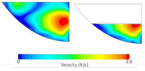
Figure 19. Illustration. Velocity distribution comparison for model 1
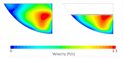
Figure 20. Illustration. Velocity distribution comparison for model 2
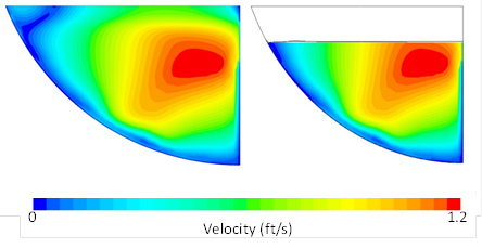
Figure 21. Illustration. Velocity distribution comparison for model 3
Building and running a two-phase full flume CFD model is time consuming. By trial and error, the appropriate flume tilt angle and flap gate opening angle are varied to achieve a uniform surface. When a nearly uniform water–air interface exists along the length of the barrel, as illustrated in figure 18, it appears possible that a single-phase model can be used to simulate the flow of water under the interface with reasonable accuracy. With this in mind, a single-phase model of the flow with a 6-inch water depth (model 2) was set up and executed. The velocity distribution results from the steady-state simulation are shown in figure 22. The same observations provided for the two-phase model shown in figure 17 are applicable for the single-phase model.

Figure 22. Illustration. Velocity distribution for the single-phase model
A comparison of the velocity distributions is provided in figure 23. The two-phase plots are cut at the 6-inch water depth, which is the same height as the single-phase flow domain. The 0.5-VOF curves are plotted on the top of the velocity contours and are slightly higher than the single-phase water flow depth. The velocity of the single-phase model is marginally larger than that of the two-phase model because in the multiphase flow model, the height of the free surface is computed, and it is slightly higher than the planned water depth. This slightly increases the cross-section area carrying water. For the purposes of defining velocities in a culvert that may inhibit fish passage for reasonably uniform flows, the small increase in water velocity when using the single-phase model is conservative. Because the single-phase flow CFD model greatly reduces computational resources and computation time, it is preferred.
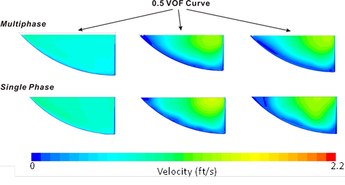
Figure 23. Illustration. Velocity comparison of the two-phase and single-phase models
Truncated Single-Phase Modeling
The single-phase model significantly reduces the simulation time. Further reductions in run times were investigated using a single-phase model with cyclic boundary conditions at the section inlet and outlet. The run time reductions are achieved by modeling a truncated 3D section of the culvert (symmetric quarter of the culvert section with corrugations from trough to another trough) rather than the full culvert length as shown in figure 24.
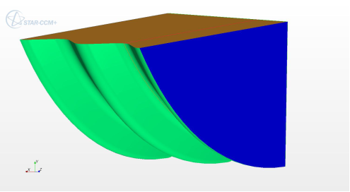
Figure 24. Illustration. Truncated section of the cyclic single-phase model
The cyclic boundary approach shortens the simulation time required to establish fully developed flow with a known mass flow rate. (With this approach, several test cases can be completed per day.) The periodic fully developed condition is achieved by creating a cyclic boundary condition where all outlet variables are mapped back to the inlet interface, except for the pressure because there is a pressure drop corresponding to the energy losses in the culvert section. The pressure jump needed to balance the pressure drop for the specified mass flow is iteratively computed by the CFD solver.
Variations in the resulting velocity distributions, and other flow parameters, of the flow field were examined by varying the base size of the mesh to obtain solutions that were effectively mesh independent.(24) Depending on the relative depth and the embedment, the number of mesh cells in the truncated model varied between 58,661 and 875,087. As previously described, more data points were taken near the boundary of the culvert than in the center of the cross-section to obtain more precise flow field data near the corrugated wall. With these observations, the truncated single-phase model with cyclic boundary conditions is used for subsequent CFD test runs. Test results indicated that for a single-phase model, the velocity simulation results of the cyclic boundary condition are similar to the non-cyclic boundary condition, which is illustrated in figure 25.
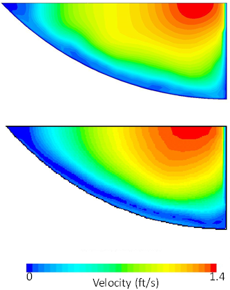
Figure 25. Illustration. Velocity distributions for non-cyclic (upper) and truncated cyclic (lower) single-phase models
To be effective, the CFD modeling must represent the roughness of the culvert walls as well as the bed material for the embedded culverts. This section describes this modeling effort as well as the methods for estimating composite roughness when more than one surface material influences the flow field.
Computing Manning's n from the CFD Analyses
The value of Manning's roughness is derived for the CFD runs using the force equilibrium equation based on figure 26 and the equation shown in figure 27. Taking a control volume of the fluid flow in an embedded pipe, the energy loss resulting from the shear stress on the wetted area (culvert walls and bed material) is reflected in a loss in pressure on the fluid flow face from the upstream end to the downstream end.

Figure 26. Illustration. Force analysis on the culvert pipe
![]()
Figure 27. Equation. Force equilibrium on a control volume
Where:
τw = Wetted perimeter shear stress, lb/ft2.
Ap = Surface area of the wetted perimeter (culvert wall and bed), ft2.
Δp = Change in pressure from one end of the control volume to the other, lb/ft2.
A = Flow cross-sectional area, ft2.
Because the pressures and areas can be derived from the CFD modeling, the wetted perimeter shear stress is computed from the equation in figure 27. Because the stresses on the wall and bed may differ with different materials, the result is the average shear stress across all the wetted surfaces.
The composite friction coefficient for a given flow condition may be estimated from the bed shear stress using the relation in figure 28.
![]()
Figure 28. Equation. Shear stress as a function of the friction factor
Where:
f = Friction factor.
ρ = Water density.
The friction factor is related to the Manning's roughness coefficient by the equation in figure 29 . The composite Manning's n value for each CFD run is determined by these relations.
![]()
Figure 29. Equation. Relation of Manning's n to friction factor
The annular corrugations of the metal culvert have been previously described. To validate that this representation provides the appropriate roughness characteristics for hydraulic modeling, several CFD runs were conducted with an 8-ft pipe flowing full. The Manning's n values from these runs were compared with those reported in HDS 5.(18) According to Hydraulic Design of Highway Culverts (HDS 5) (appendix B, figure B.3), the Manning's n for 6- by 2-inch annular corrugations on an 8-ft diameter CSP is 0.0344. This value is for high-flow design conditions, which are defined to be when Q/D2.5 equals 4.0 ft0.5/s.
The full-flow CFD runs using a 16-ft-long model resulted in a Manning's n value of 0.0325. This is less than 6 percent lower than the recommended value of HDS 5. Prior to running the 16-ft-long model, shorter models of 1 and 2 ft were also tested with CFD. The resulting Manning's n values were slightly lower than for the 16-ft model.
It should also be noted that the Q/D2.5 value for the CFD is 0.29 ft0.5/s, which is much lower than the values assumed for HDS 5. Although this indicates lower flow intensity, this difference is not expected to affect the computation of the Manning's n.
Characterizing bed roughness for natural rivers and streams within CFD models is challenging.(25) In the flume test runs, the culvert bed material was coarse gravel with a mean diameter, D50, equal to 0.472 inches. For this size of material, the gravel bed boundary cannot simply be treated as a rough wall using wall functions because the centroid of the near wall computational cell must be at a position that is greater than the roughness height. For this size of gravel, the near wall mesh would be far too large for the analysis results to be mesh independent, as is required. The following three options to model flow parallel to a porous gravel bed were considered:(26)
A justification for simulating the roughness of a gravel bed using a porous media configuration is that in a gravel bed, there is shear induced flow within the bed. Depending upon the permeability of the bed material, various levels of sub-surface flow are possible. The porous media approach not only provides a method to simulate surface roughness, but it also includes the effects of the flow within the bed structure.
To model flow through a porous media, the STAR-CCM+ User Guide notes that it is not the details of the internal flow in the porous region that are of interest, but rather the macroscopic effect of the porous medium on the overall fluid flow.(27) The effect of the porous medium on the flow is defined using lumped parameters that are typically taken to be resistance coefficients for two sink terms in the momentum equation. One is linearly proportional to velocity and the other proportional to velocity squared. These parameters account for the effect of the distributed surface area of the porous media as a flow resistance on the bulk flow in the porous media and, consequently, affect the flow that borders the porous region. If the porous region represents a gravel bed in a culvert, then it should have the effect of a very rough wall with a small slip condition at the interface that is determined by the flow resistance of the porous media.
Various CFD tests were conducted to determine whether a porous media model appears to be a viable way to model large-diameter gravel in the bed of a culvert. Some of the results obtained appeared reasonable, while others appeared to be physically unrealistic. The physically unrealistic results did not appear to capture the viscous transport of momentum from the open-flow region into the porous-flow region. This result was most likely a consequence of mesh refinement in the vicinity of the porous media interface. Because a boundary layer with a small slip condition does exist at the porous media interface, and wall functions for this model are not available to determine shear stress at the interface, using a sufficiently refined grid to resolve the velocity profile near the interface is important.
An additional difficulty with using the porous media approach was that comparisons would be made to physical modeling results and not field measurements. Because the physical modeling of the bed material was achieved by gluing one layer of the gravel on the bottom of the flume, there would be no flow through the bed material, leaving the porous media approach unsuitable for this project.
Another method was to model the gravel roughness by simulating the top layer of the gravel by detailed contouring. The CAD model for the contoured bed was created in Pro-ENGINEER. The challenge in selecting the appropriate contouring to mimic a gravel bed is the potential for introducing numerical error after importing the CAD bed model into STAR-CCM+. Because numerical errors may be caused by sharp angles between grids, two quarter-circular arcs with the appropriate diameter are used to create smooth connections. Figure 30 illustrates the method of creating a D50 equal to 0.944 inches. Figure 31 shows a part of the model with the contours simulating a gravel bed. This approach for representing the gravel bed was used for the embedded culvert runs listed in table 4 through table 7.
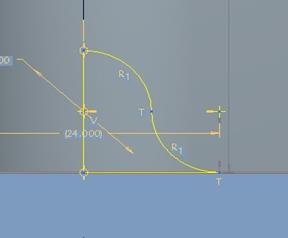
Figure 30. Illustration. Gravel contour method in the CAD model
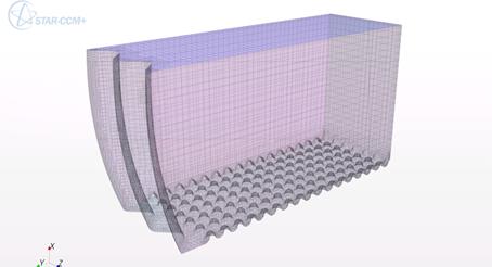
Figure 31. Illustration. Gravel bed surface created by contouring
The final method was to model the gravel roughness as one or more layers of uniform spheres. The CAD model for this approach was created in SolidWorks. Spheres with diameters (D50 values) of 0.39, 0.87, 1.34, and 2.28 inches were used in CFD runs primarily to refine the modeling estimates of Manning's n and for estimating composite roughness values. It was found that when the particle size is small, the porosity of the bed material is not properly simulated with a single layer of particles, as shown in figure 32. This may be because the boundary below is a smooth, solid surface and does not represent a gravel bed well. To address this problem, a second layer of particles, as shown in figure 33, was added and the results compared with the single layer runs. A single layer worked well for the two larger diameter spheres, but a double layer was needed for the 0.39 and 0.87 inch D50 runs.
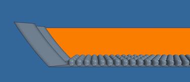
Figure 32. Illustration. Single sphere layer for bed roughness
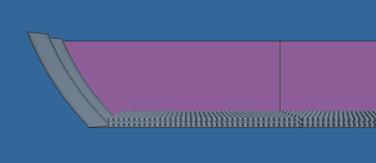
Figure 33. Illustration. Double sphere layer for bed roughness
Comparison With Empirical Estimates of Bed Roughness
Results from the CFD modeling may be compared with Manning's roughness estimates using empirical relations such as the Blodgett equation for bed roughness shown in figure 34.(1) Other relations are available and discussed in Aquatic Organism Passage Design Guidelines for Culverts (HEC 26), but the Blodgett equation performs well for the range of conditions considered in this study.(1)

Figure 34. Equation. Blodgett's equation for bed roughness
Where:
α = 0.262 for customary units and 0.319 for metric units.
Because the CFD roughness values are composite values (bed and culvert wall), the bed material roughness was not directly estimated in the CFD runs and could not be compared with the Blodgett estimates. The ability of CFD to represent the bed roughness is assessed indirectly through comparison of overall composite roughness.
Further complicating the comparison is that the CFD representation of the bed material using the spheres includes particles of only one size. The Blodgett equation uses the D50 as a defining characteristic of the bed material but anticipates that the bed material has particles both smaller and larger than this value.
To fully evaluate the CFD modeling of roughness, the composite roughness of an embedded culvert must consider the combined effect of the bed material and the culvert material. The CFD computation method presented previously directly produces a composite roughness because the combined shear force from the bed and culvert wall is jointly considered. These CFD estimates of the composite Manning's n are compared with composite Manning's n estimates from each of three compositing methods that use a separate value of roughness for the culvert wall and the Blodgett estimate of bed material roughness.
A detailed description of compositing methods is provided in appendix C of HEC 26.(1) It includes three alternative methods. One approach is a simple weighting of n values based on wetted perimeter. This approach is used by the software tool FishXing and is described by the equation in figure 35.

Figure 35. Equation. Linear compositing
Where:
nc = Composited n-value for the culvert.
Pb = Wetted perimeter of the bed material in the culvert.
nb= n-value of the bed material in the culvert.
Pw= Wetted perimeter of the culvert walls above the bed material.
nw= n-value of the culvert material.
A second approach is applied by the software tools HY-8 and Hydrologic Engineering Centers River Analysis System (HEC-RAS), described in HDS 5, and recommended by Tullis.(28, 18, 29) It uses an exponent other than unity in weighting the roughness values. This approach is described by the equation in figure 36.

Figure 36. Equation. Exponential compositing
A third approach considers that the energy lost to friction along the wetted perimeter is a function of the roughness and the boundary force applied to the boundary. This approach recognizes that for open channel flow, the hydrostatic forces on the culvert side wall are not equivalent to those on the bed. The approach incorporates this concept by introducing a wall shape coefficient in the weighting that is fully described in HEC 26.(1) The equation is presented in figure 37.

Figure 37. Equation. Linear compositing with wall shape coefficient
Where:
cy = Wall shape coefficient, between 0 and 1.
The wall shape coefficient is 0.5 for a box culvert. Because the shallow flows in embedded culverts approximate a rectangular shape for the flow field, the 0.5 value for wall shape coefficient is appropriate for these conditions.
A total of 18 CFD runs were completed to compare estimates of composite Manning's roughness. These included three flow depths, three particle sizes, and two levels of embedment within an 8-ft diameter CSP culvert. The bed material was represented using the spherical approach described previously with sphere diameters of 0.39, 0.87, and 1.34 inches. All runs used the same average flow velocity. From each of these runs, a composite Manning's n was developed using the previously described methodology.
These CFD-derived values are compared with values derived from the HDS 5 value of 0.0344 for the culvert wall and Blodgett's equation for the bed material given the D50 and flow depth for each case. The individual material values were then composited using each of the three methodologies outlined. The root mean square (RMS) difference between the CFD and analytically derived values was computed.
The RMS difference ranged from 0.0040 for the linear compositing method with the wall shape coefficient to 0.0047 for the exponential compositing method. These differences range from 12 to 14 percent of the HDS 5 Manning's n value of 0.0344 for the culvert wall. Figure 38 shows a plot of the CFD values versus the HDS 5/Blodgett values using the exponential compositing method. Although the data are scattered, the CFD values tend to underestimate the analytically derived estimates.
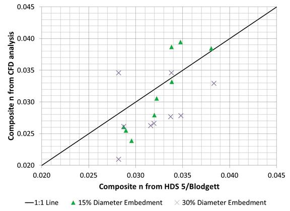
Figure 38. Graph. Comparison of composite Manning's n
Several factors may contribute to the differences in composite Manning's n computed from the CFD modeling and the analytical methods. These include the compositing method, the use of the HDS 5 culvert value, the accuracy of the Blodgett equation for bed material roughness, and the CFD surface modeling approach. Because the latter has already been addressed, variations in the other three factors are evaluated.
Alternative values of the culvert wall and bed material roughness were selected, and the resulting composite Manning's n from each of the three compositing methods was computed. Table 3 summarizes the RMS differences for these analytical scenarios compared with the CFD results.
The first row in the table summarizes the results when using the HDS 5 culvert value and Blodgett estimates without adjustment. This is the scenario discussed previously. In the second scenario summarized in the table, the HDS 5 culvert value of 0.0344 is replaced with the Manning's n from the CFD modeling of the culvert flowing full without any embedment (0.0325). The third scenario retains the 0.0325 value for the culvert wall and employs a multiplier on the Blodgett estimates for the bed material roughness as shown in figure 39. The multiplier was selected to minimize the RMS difference. The Blodgett multiplier is intended to compensate for any systematic under or over estimate of the bed material Manning's n. The resulting multiplier was 0.93, meaning that when all Blodgett estimates are reduced by 7 percent, the smallest RMS difference is obtained.

Figure 39. Equation. Blodgett's equation for bed roughness with multiplier
Where:
k = Blodgett multiplier.
Table 3 . Summary of composite Manning's n analyses.
Blodgett Multiplier, k |
Culvert Wall Manning's n |
RMS Difference: Linear |
RMS Difference: Exponential |
RMS Difference: Linear with Wall Coefficient |
|---|---|---|---|---|
1.0 |
0.0344 |
0.0046 |
0.0047 |
0.0040 |
1.0 |
0.0325 |
0.0044 |
0.0044 |
0.0042 |
0.93 |
0.0325 |
0.0041 |
0.0041 |
0.0040 |
Among the scenarios analyzed and compositing methods considered, there are no clear conclusions about the superiority of one approach over another. Although the RMS differences are lower with the wall coefficient method in all three scenarios, the differences between the three methods are not significant. Therefore, the exponential method is recommended because it already enjoys widespread acceptance.
Test matrices were developed to achieve several project objectives. All CFD runs are labeled as CpqrrVsDt where: 1) p represents the diameter of the culvert in feet, 2) q designates whether the run is a symmetrical half section (H) or full section (F), 3) rr represents the embedment level (in percent of the culvert diameter), 4) s represents a velocity index from lowest to highest in the matrix, and 5) t represents the depth index from lowest to highest in the matrix. For example, C6F15V2D3 is a 6-ft-diameter full-section run with the embedment at 15 percent of the diameter. The depth and velocity for the run are the second and third values, respectively, from the matrix.
The objective of matrix CFD1 (see table 4) is to validate CFD results by comparing the modeled velocity fields with those measured in the experimental flume. All runs are based on a symmetrical half-section 3-ft corrugated metal pipe with 3-inch by 1-inch corrugations. Two velocities (discharges) were tested at each embedment and flow depth. Flow depths of 4.5, 6, and 9 inches represented 12, 16, and 25 percent of the culvert diameter, respectively. Embedment of 0 inches represents the case with no embedment, while embedment depths of 5.4 inches and 10.8 inches represent 15 and 30 percent of the culvert diameter, respectively. In the 15- and 30-percent embedment runs, a bed material with a D50 of 0.472 inches was simulated using the bed contouring approach.
Table 4. Matrix CFD1 for 3-ft CMP (half section).
Run ID |
Flow Depth (inches) |
Embedment (inches) |
Flow Velocity (ft/s) |
|---|---|---|---|
C3H00V1D1 |
4.5 |
0 |
0.71 |
C3H00V1D2 |
6 |
||
C3H00V1D3 |
9 |
||
C3H00V2D1 |
4.5 |
0 |
1.1 |
C3H00V2D2 |
6 |
||
C3H00V2D3 |
9 |
||
C3H15V1D1 |
4.5 |
5.4 |
0.71 |
C3H15V1D2 |
6 |
||
C3H15V1D3 |
9 |
||
C3H15V2D1 |
4.5 |
5.4 |
1.1 |
C3H15V2D2 |
6 |
||
C3H15V2D3 |
9 |
||
C3H30V1D1 |
4.5 |
10.8 |
0.71 |
C3H30V1D2 |
6 |
||
C3H30V1D3 |
9 |
||
C3H30V2D1 |
4.5 |
10.8 |
1.1 |
C3H30V2D2 |
6 |
||
C3H30V2D3 |
9 |
The objectives of matrix CFD2 (see table 5) are to validate CFD results by comparing the half-section computations with full-section computations. All runs are based on a 3-ft corrugated metal pipe with 3-inch by 1-inch corrugations. Two velocities (discharges) were tested at each embedment and flow depth. Flow depths of 4.5, 5, 6, 7, 8, 9, and 10 inches were tested. Embedment of 0 inches represents the case with no embedment, while embedment depths of 5.4 inches and 10.8 inches represent 15 and 30 percent of the culvert diameter, respectively. For the 15 and 30 percent embedment runs, a bed material with a D50 of 0.472 inches was simulated using the bed contouring approach.
Table 5. Matrix CFD2 for 3-ft CMP (full section).
Run ID |
Flow Depth (inches) |
Embedment (inches) |
Flow Velocity (ft/s) |
|---|---|---|---|
C3F00V1D1 |
4.5 |
0 |
0.71 |
C3F00V1D2 |
5 |
||
C3F00V1D3 |
6 |
||
C3F00V1D4 |
7 |
||
C3F00V1D5 |
8 |
||
C3F00V1D6 |
9 |
||
C3F00V1D7 |
10 |
||
C3F00V2D1 |
4.5 |
0 |
1.1 |
C3F00V2D2 |
5 |
||
C3F00V2D3 |
6 |
||
C3F00V2D4 |
7 |
||
C3F00V2D5 |
8 |
||
C3F00V2D6 |
9 |
||
C3F00V2D7 |
10 |
||
C3F15V1D1 |
4.5 |
5.4 |
0.71 |
C3F15V1D2 |
5 |
||
C3F15V1D3 |
6 |
||
C3F15V1D4 |
7 |
||
C3F15V1D5 |
8 |
||
C3F15V1D6 |
9 |
||
C3F15V1D7 |
10 |
||
C3F15V2D1 |
4.5 |
5.4 |
1.1 |
C3F15V2D2 |
5 |
||
C3F15V2D3 |
6 |
||
C3F15V2D4 |
7 |
||
C3F15V2D5 |
8 |
||
C3F15V2D6 |
9 |
||
C3F15V2D7 |
10 |
||
C3F30V1D1 |
4.5 |
10.8 |
0.71 |
C3F30V1D2 |
5 |
||
C3F30V1D3 |
6 |
||
C3F30V1D4 |
7 |
||
C3F30V1D5 |
8 |
||
C3F30V1D6 |
9 |
||
C3F30V1D7 |
10 |
||
C3F30V2D1 |
4.5 |
10.8 |
1.1 |
C3F30V2D2 |
5 |
||
C3F30V2D3 |
6 |
||
C3F30V2D4 |
7 |
||
C3F30V2D5 |
8 |
||
C3F30V2D6 |
9 |
||
C3F30V2D7 |
10 |
The objective of matrix CFD3 (see table 6) is to consider scaled roughness and slope. All runs are based on a 6-ft corrugated metal pipe with 6-inch by 2-inch corrugations. Two velocities (discharges) were tested at each embedment and flow depth. Flow depths of 6, 12, and 18 inches represented 8, 16, and 25 percent of the culvert diameter, respectively. All runs are models of full culvert sections. Embedment of zero inches represents the case with no embedment, while embedment depths of 10.8 inches and 21.6 inches represent 15 and 30 percent of the culvert diameter, respectively. In the 15- and 30-percent embedment runs, a bed material with a D50 of 0.944 inches was simulated using the bed contouring approach. Roughness for the CMP and embedment material is based on detailed representation of the CMP and the contoured bed material. The 6-ft culvert runs are scaled from the 3-ft runs based on the Froude number.
Table 6. Matrix CFD3 for 6-ft CMP.
Run ID |
Flow Depth (inches) |
Embedment (inches) |
Flow Velocity (ft/s) |
|---|---|---|---|
C6F00V1D1 |
6 |
0 |
1.0 |
C6F00V1D2 |
12 |
||
C6F00V1D3 |
18 |
||
C6F00V2D1 |
6 |
0 |
1.56 |
C6F00V2D2 |
12 |
||
C6F00V2D3 |
18 |
||
C6F15V1D1 |
6 |
10.8 |
1.0 |
C6F15V1D2 |
12 |
||
C6F15V1D3 |
18 |
||
C6F15V2D1 |
6 |
10.8 |
1.56 |
C6F15V2D2 |
12 |
||
C6F15V2D3 |
18 |
||
C6F30V1D1 |
6 |
21.6 |
1.0 |
C6F30V1D2 |
12 |
||
C6F30V1D3 |
18 |
||
C6F30V2D1 |
6 |
21.6 |
1.56 |
C6F30V2D2 |
12 |
||
C6F30V2D3 |
18 |
The objective of matrix CFD4 (see table 7) is to investigate velocity distributions at a large (prototype) scale. All runs are based on an 8-ft corrugated metal pipe with 6- by 2-inch corrugations. Two velocities (discharges) were tested at each embedment and flow depth. Flow depths of 7.7, 15.4, and 24 inches represented 8, 16, and 25 percent of the culvert diameter, respectively. The velocities were chosen to represent a realistic range of velocities of concern for fish passage at this scale. All runs are models of full culvert sections. Embedment of 0 inches represents the case with no embedment, while embedment depths of 14.4 and 28.8 inches represent 15 and 30 percent of the culvert diameter, respectively. For the 15- and 30-percent embedment runs, a bed material with a D50 of 0.944 inches was simulated using the bed contouring approach. The 8-ft culvert runs are not scaled from the 3-ft runs.
Table 7. Matrix CFD4 for 8-ft CMP.
Run ID |
Flow Depth (inches) |
Embedment (inches) |
Flow Velocity (ft/s) |
|---|---|---|---|
C8F00V1D1 |
7.7 |
0.0 |
1.0 |
C8F00V1D2 |
15.4 |
||
C8F00V1D3 |
24.0 |
||
C8F00V2D1 |
7.7 |
0.0 |
3.0 |
C8F00V2D2 |
15.4 |
||
C8F00V2D3 |
24.0 |
||
C8F15V1D1 |
7.7 |
14.4 |
1.0 |
C8F15V1D2 |
15.4 |
||
C8F15V1D3 |
24.0 |
||
C8F15V2D1 |
7.7 |
14.4 |
3.0 |
C8F15V2D2 |
15.4 |
||
C8F15V2D3 |
24.0 |
||
C8F30V1D1 |
7.7 |
28.8 |
1.0 |
C8F30V1D2 |
15.4 |
||
C8F30V1D3 |
24.0 |
||
C8F30V2D1 |
7.7 |
28.8 |
3.0 |
C8F30V2D2 |
15.4 |
||
C8F30V2D3 |
24.0 |
The data from physical modeling provided a reliable means to calibrate and validate the CFD modeling. For each flow condition specified in the test matrix for physical modeling (see table 1), comparisons were made with velocity data from CFD modeling (matrix CFD1). The physical modeling included runs with 3 water depths, 2 flow velocities, and 3 embedment levels to produce 18 data sets.
Velocities measured in the flume by PIV and estimated by the CFD model were compared using the root mean square error (RMSE) of data points measured/computed in the cross-section. (The PIV measurements from the physical model are considered to be the "correct" values.) Interpolating both data sources to a 0.197- by 0.197-inch grid, the RMSE is defined in the equation in figure 40.
Where:
RMSE = Root mean square error in velocity, ft/s.
Vi,1 = Velocity at the ith point in the cross-section as computed by CFD, ft/s.
Vi,2 = Velocity at the ith point in the cross-section as measured by PIV, ft/s.
n = Number of velocity measurements available in the cross-section.
A relative percentage error is defined in the equation in figure 41. The relative errors for each run are listed in table 8 and range from 10.3 to 24.0 percent.

Figure 41. Equation. Relative error
Where:
RE = Relative error, dimensionless.
Va = Average velocity (nominal) in the cross-section, ft/s.
Color-coded velocity plots provide visual evidence of the agreement between CFD simulations and the physical experiments. The condition with zero embedment with a flow depth of 4.5 inches and a velocity of 0.71 ft/s (run F3H00V1D1) is shown in figure 42. Similarly, the condition with a depth of 9 inches and a velocity of 1.1 ft/s (run F3H00V2D3) is shown in figure 43. Both show good agreement.
Additional runs were completed with embedment at 15 and 30 percent of the culvert diameter. Results for the 30-percent embedment level with a flow depth of 4.5 inches and a velocity of 0.71 ft/s (run F3H30V1D1) are shown in figure 44. Similarly, the condition with a depth of 9 inches and a velocity of 1.1 ft/s (run F3H30V2D3) is shown in figure 45. Both show good agreement.
The gridded point velocities were averaged to determine the average cross-sectional velocity for each run as estimated in the flume by PIV and in the CFD modeling. These are compared in figure 46 and show reasonable agreement. This comparison supports the adequacy of CFD modeling for the purposes of this project.
ADV measurements, limited by the relatively small measurable area in the culvert cross-section (especially in shallow conditions), did not compare very well with the average velocity from CFD results. These limits were discussed previously.Table 8. Relative error for cross-section velocity measurements.
Flume Run ID |
CFD Run ID |
Embedment (inches) |
Velocity (ft/s) |
Water depth (inches) |
Relative |
|---|---|---|---|---|---|
F3H00V1D1 |
C3H00V1D1 |
0 |
0.71 |
4.5 |
24.0 |
F3H00V1D2 |
C3H00V1D2 |
0 |
0.71 |
6 |
20.0 |
F3H00V1D3 |
C3H00V1D3 |
0 |
0.71 |
9 |
20.0 |
F3H00V2D1 |
C3H00V2D1 |
0 |
1.1 |
4.5 |
28.4 |
F3H00V2D2 |
C3H00V2D2 |
0 |
1.1 |
6 |
18.6 |
F3H00V2D3 |
C3H00V2D3 |
0 |
1.1 |
9 |
21.8 |
F3H15V1D1 |
C3H15V1D1 |
5.4 |
0.71 |
4.5 |
12.3 |
F3H15V1D2 |
C3H15V1D2 |
5.4 |
0.71 |
6 |
20.9 |
F3H15V1D3 |
C3H15V1D3 |
5.4 |
0.71 |
9 |
10.6 |
F3H15V2D1 |
C3H15V2D1 |
5.4 |
1.1 |
4.5 |
10.3 |
F3H15V2D2 |
C3H15V2D2 |
5.4 |
1.1 |
6 |
14.5 |
F3H15V2D3 |
C3H15V2D3 |
5.4 |
1.1 |
9 |
10.6 |
F3H30V1D1 |
C3H30V1D1 |
10.8 |
0.71 |
4.5 |
20.3 |
F3H30V1D2 |
C3H30V1D2 |
10.8 |
0.71 |
6 |
18.2 |
F3H30V1D3 |
C3H30V1D3 |
10.8 |
0.71 |
9 |
12.8 |
F3H30V2D1 |
C3H30V2D1 |
10.8 |
1.1 |
4.5 |
19.9 |
F3H30V2D2 |
C3H30V2D2 |
10.8 |
1.1 |
6 |
16.4 |
F3H30V2D3 |
C3H30V2D3 |
10.8 |
1.1 |
9 |
11.2 |
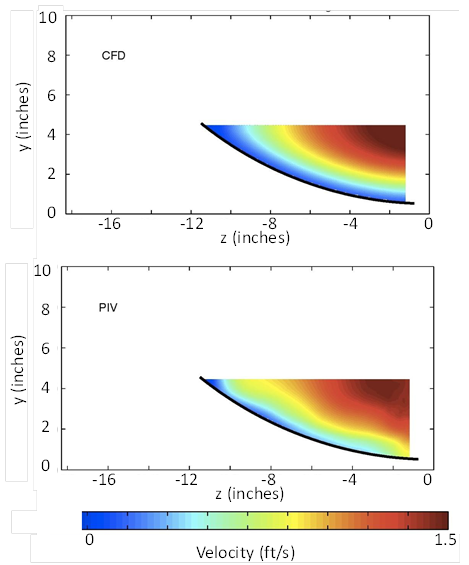
Figure 42. Illustration. Comparison of CFD and PIV results for run F3H00V1D1
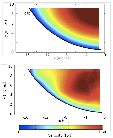
Figure 43. Illustration. Comparison of CFD and PIV results for run F3H00V2D3
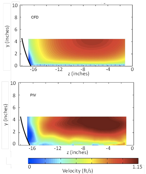
Figure 44. Illustration. Comparison of CFD and PIV results for run F3H30V1D1
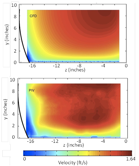
Figure 45. Illustration. Comparison of CFD and PIV results for run F3H00V2D3
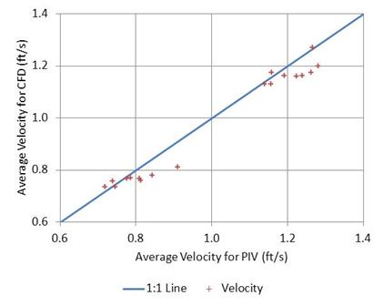
Figure 46. Graph. Comparison of CFD and PIV mean velocities
Vertical and Horizontal Slice Comparisons
Because the proposed methodology is based on depth-averaged vertical slices, comparisons between the methods by vertical slices were completed. Because the ADV probe cannot measure reliably within a relatively large area near the walls, the comparison is primarily between the PIV measurements and CFD results. However, ADV data in the area where the probe provided good readings are included for comparison.
The error in measurements, for either vertical or horizontal slices, is defined in figure 47:

Figure 47. Equation. Slice RMSE
Where:
RMSEx = Root mean square difference in velocity for the xth slice, ft/s.
Vx,i,1 = Velocity at the ith point in the xth slice as computed by CFD, ft/s.
Vx,i,2 = Velocity at the ith point in the xth slice as measured by PIV, ft/s.
nx = Number of velocity measurements in the xth slice.
A relative percentage error is used as a normalized measure and is defined in figure 48:

Figure 48. Equation. Relative error in the xth slice
Where:
REx = Relative error in the xth slice, dimensionless.
Vx,max = Maximum point velocity measured (PIV) in the xth slice, ft/s.
Vx,min = Minimum point velocity measured (PIV) in the xth slice, ft/s.
Figure 49 shows a vertical profile (slice) comparison for flume run F3H00V1D1 (no embedment). The vertical slice shown is taken 3.94 inches from the centerline of the 3-ft culvert. Similarly, figure 50 shows the same comparison for flume run F3H00V2D3.
A width averaged (horizontal slice) comparison was also completed. Figure 51 shows a horizontal profile comparison for flume run F3H00V1D1 (no embedment). The horizontal slice shown is taken 3.94 inches from the bottom of the 3-ft culvert. Similarly, figure 52 shows the same comparison for flume run F3H00V2D3. The relative errors for each of the runs compared are listed in table 9 and range from 7.8 to 18.4 percent.
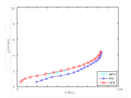
Figure 49. Graph. Vertical slice velocity comparison for flume run F3H00V1D1
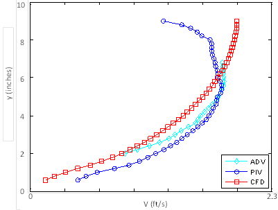
Figure 50. Graph. Vertical slice velocity comparison for flume run F3H00V2D3
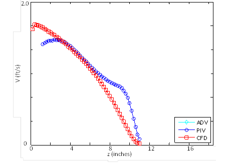
Figure 51. Graph. Horizontal slice velocity comparison for flume run F3H00V1D1
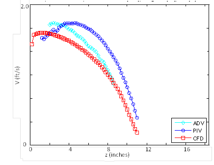
Figure 52. Graph. Horizontal slice velocity comparison for flume run F3H00V2D3
Table 9. Relative error for slice velocity measurements.
Flume Run ID |
CFD Run ID |
Embedment (inches) |
Velocity (ft/s) |
Water Depth (inches) |
Vertical Slice Relative |
Horizontal Slice Relative |
|---|---|---|---|---|---|---|
F3H00V1D1 |
C3H00V1D1 |
0 |
0.71 |
4.5 |
16.5 |
11.9 |
F3H00V1D2 |
C3H00V1D2 |
0 |
0.71 |
6 |
16.4 |
8.4 |
F3H00V1D3 |
C3H00V1D3 |
0 |
0.71 |
9 |
12.2 |
15.8 |
F3H00V2D1 |
C3H00V2D1 |
0 |
1.1 |
4.5 |
13.8 |
16.1 |
F3H00V2D2 |
C3H00V2D2 |
0 |
1.1 |
6 |
14.0 |
7.8 |
F3H00V2D3 |
C3H00V2D3 |
0 |
1.1 |
9 |
14.3 |
18.4 |
The CFD data are in good agreement with experimental measurements using PIV. The differences may be attributed to one or more of the following reasons:
It is also noted that the CFD measurements are generally taken in the trough section of the corrugation rather than on the inner section of the corrugation. This approach results in a larger cross-sectional area than would be expected using nominal culvert dimensions because the trough extends beyond the nominal pipe diameter. With the larger cross-sectional area and a given flow, the average velocity is somewhat smaller than would be nominally computed.
In the following analyses, the magnitude of the velocity vectors at each point is taken as the velocity for that point. In most of the culvert cross-section, the direction of the vector is aligned with the longitudinal flow. However, in the trough area, the velocity vectors point in many directions because of the turbulence caused by the corrugations. The magnitude of these vectors is small in comparison with those aligned with the flow.
SYMETRICAL HALF VERSUS FULL CULVERT MODELS
Although useful for comparing CFD modeling with physical modeling in the flume, the symmetrical half sections are not appropriate for evaluating the velocity distribution across a culvert section. Figure 53 presents a comparison of the half-section and full-section runs for the 6-inch depth with the 0.71 ft/s velocity for the 0- and 30-percent embedment conditions. At the centerline, where there is a wall in the half section, the velocity is significantly reduced for the half-section runs compared with the full-section runs. Other flow conditions behave in a similar manner. Only full-section runs are evaluated further for development of a design methodology.
With the CFD modeling, there is an opportunity to evaluate many more and larger models than is feasible in the laboratory flume. Test runs with 6- and 8-ft diameter corrugated metal pipes were conducted as previously described in test matrices CFD3 and CFD4, respectively. The sensitivity to parameters such as size and corrugation dimensions is tested.
The 6-ft diameter corrugated metal pipe is scaled up from the 3-ft model based on the Froude number and a 2:1 length ratio. The laboratory model culvert corrugation is 3 inches by 1 inch, while the 6-ft model has 6- by 2-inch corrugations. The embedment and water depths were all twice the size of the flume model. Two velocities were tested in the flume, 0.71 ft/s and 1.1 ft/s, which correspond to the larger scale model velocities of 1.0 and 1.56 ft/s, respectively. The laboratory bed material D50 equals 0.472 inches; therefore, the larger-scale bed material D50 equals 0.944 inches. For the 6-ft diameter model, the base size of the meshing increased to twice that for the 3-ft culvert in the CFD modeling. Because the model geometry is larger than the previous model and simulation speed is influenced by a larger mesh, run times were extended.
Because the proposed fish passage design is based on the depth-averaged velocities in various slices across the width of the culvert, the results of the original 3-ft diameter model and the scaled 6-ft diameter model are compared. To adjust for scale, the velocity is normalized by average velocity, and position is normalized by the culvert diameter. Figure 54 through figure 56 illustrate the comparison for embedment elevations of 0, 15, and 30 percent of the culvert diameter, respectively.
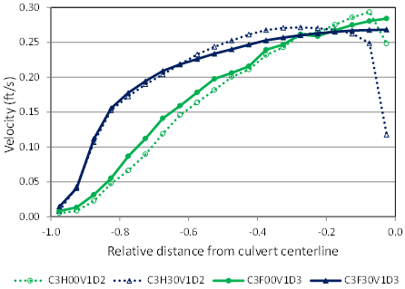
Figure 53. Graph. Selected comparison of half- and full-section CFD runs
The CFD culvert model was also applied to an 8-ft diameter corrugated metal pipe. Many of the length parameters were scaled up from the 3-ft CMP tests. Flow depths were maintained at 8, 16, and 25 percent of the culvert diameter equaling to 7.7, 15.4, and 24 inches, respectively. Embedment was tested at 0, 15, and 30 percent of the culvert diameter.
The velocities were chosen to be within the range of concern for fish passage at this scale, not based on Froude number similitude. Two velocities were tested for each geometric configuration: 1.0 and 3.0 ft/s. The roughness elements-corrugations and bed material-were the same as those used for the 6-ft model. The bed was modeled to simulate gravel with a D50 equal to 0.944 inches, and the corrugations were 6 by 2 inches.
The resulting velocity distributions are displayed in figure 57, figure 58, and figure 59. These plots demonstrate that there are steep velocity gradients close to the bed and walls, which is characteristic of turbulent flow with fully developed boundary layers.
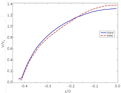
Figure 54. Graph. Comparison of 6- and 3-ft models with no embedment
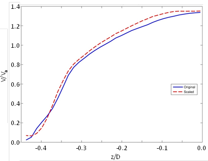
Figure 55. Graph. Comparison of 6- and 3-ft models with 15-percent embedment
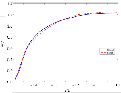
Figure 56. Graph. Comparison of 6- and 3-ft models with 30-percent embedment
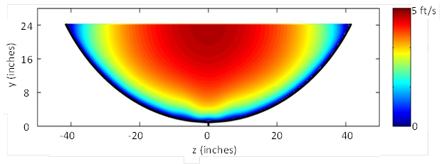
Figure 57. Illustration. Velocities for run C8F00V2D3 (no embedment)
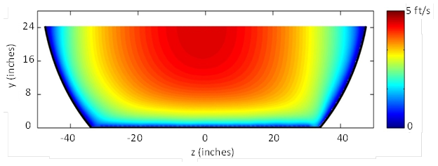
Figure 58. Illustration. Velocities for run C8F15V2D3 (15-percent embedment)
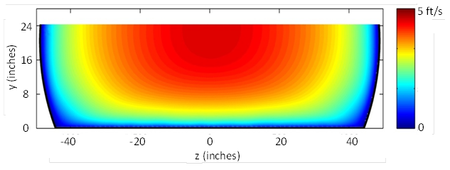
Figure 59. Illustration. Velocities for run C8F30V2D3 (30-percent embedment)