U.S. Department of Transportation
Federal Highway Administration
1200 New Jersey Avenue, SE
Washington, DC 20590
202-366-4000
Federal Highway Administration Research and Technology
Coordinating, Developing, and Delivering Highway Transportation Innovations
| REPORT |
| This report is an archived publication and may contain dated technical, contact, and link information |
|
| Publication Number: FHWA-HRT-14-064 Date: August 2014 |
Publication Number: FHWA-HRT-14-064 Date: August 2014 |
To achieve the research goal of developing design tools to estimate the velocity distribution in an embedded culvert, a means of characterizing the velocity distribution is needed. House et al. used regression techniques to estimate the percentage of a stream cross-section less than or equal to a given velocity.(9) This work is limited to the relatively narrow range of observed conditions used in the regression. Chiu and Chiou and then Chiu describe a mathematical model for velocity distribution that may have broader application and was adapted for this research.(30,31)
In the mathematical model described by Chiu and Chiou, the Cartesian coordinate system is replaced with a curvilinear system that aligns with the equal velocity curves (isovels) in a channel as shown in figure 60 and figure 61.(30) In this coordinate system, Y and Z are replaced by ξ and η, where the ξ curves represent the isovels. ymax represents the flow depth at the deepest point in the channel, typically the centerline, and Bi represents the top width of the flow to the left (i = 1) and right (i = 2) of the centerline, allowing for consideration of an asymmetrical channel. The difference between the two figures is the value of the parameter ε. In figure 60, it is non-negative (not shown), indicating that velocity continues to increase at the centerline as the water surface is approached. It is negative in figure 61, when the peak velocity is located below the water surface.
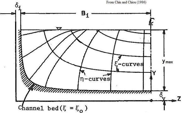
Figure 60. Illustration. Isovel coordinate system (ε ≥ 0)
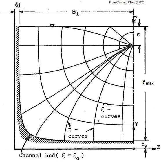
Figure 61. Illustration. Isovel coordinate system (ε < 0)
The primary isovels can be estimated as shown in figure 62:
![]()
Figure 62. Equation. Isovel equation
Where:
ξ = Primary isovel coordinate value.
Y = Normalized Cartesian coordinate in the vertical direction.
Z = Normalized Cartesian coordinate in the horizontal direction.
βi = Velocity distribution parameter.
The normalized Cartesian coordinates are computed from the equations in figure 63 and figure 64.

Figure 63. Equation. Normalized Y coordinate
Where:
y = Vertical distance, ft.
δy = Velocity distribution parameter as shown in figure 60 and figure 61, ft.
ymax = Water depth at the y-axis (culvert centerline), ft.
ε = Velocity distribution parameter as shown in figure 60 and figure 61, ft.

Figure 64. Equation. Normalized Z coordinate
Where:
z = Horizontal distance from the culvert centerline, ft.
δi = Velocity distribution parameter as shown in figure 60 and figure 61, ft.
βi = Transverse distance on the water surface to the left (i = 1) and right (i =2), ft.
The parameters δy, δi, and βi primarily control the shape of the zero-velocity isovel and the isovels near the bed and sides of the channel. The parameter ε primarily influences the higher isovels closer to the surface in the center of the channel.
Figure 65 presents Chiu's relation for computing the velocity at any point in the channel based on the maximum velocity in the channel and the ξ value.(31)

Figure 65. Equation. Point velocity
Where:
V = Point velocity for the ξ isovel, ft/s.
Vmax = Maximum point velocity in the channel cross-section, ft/s.
M = Velocity distribution parameter.
ξo = Minimum value for the ξ coordinate.
ξmax = Maximum value for the ξ coordinate.
Using the equations in figure 62 through figure 65, the velocity at any point in the channel can be estimated if the velocity distribution parameters can be determined. Zhai applied regression techniques to the CFD modeling results for the 3-ft culvert presented earlier to estimate M,ε,βi, δi, and δy.(32) However, Zhai's analysis resulted in parameter values inconsistent with the physical meaning of several of the parameters. Zhai also did not provide any guidance on estimating these parameters for design purposes.
Figure 66 through figure 68 illustrate the depth-averaged velocity distributions from the CFD modeling for no embedment, 15-percent embedment, and 30-percent embedment, respectively, for the V1 conditions. These figures are the normalized such that the abscissa is the distance from the culvert centerline, z (negative indicates measurement to the left of the centerline), relative to the water surface width from the centerline to the left edge of the water surface, B1. The ordinate axis is the vertically averaged velocity at that location, V, relative to the average velocity in the culvert, Va. Similar patterns were observed for the higher V2 velocity.
Immediately apparent is the greater profile variation for the no-embedment runs. Conversely, the velocity distributions are virtually identical for the 30-percent embedment runs where the channel cross-sections approximate a rectangular shape. Figure 69 summarizes a cross-comparison for the intermediate depth, D4, illustrating the differences in the velocity distributions with embedment. Reasonable estimates of the velocity distribution parameters are necessary to capture these variations.
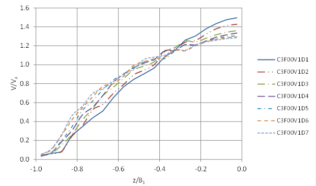
Figure 66. Graph. Vertical slice velocity for no embedment (V1)
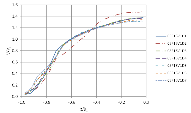
Figure 67. Graph. Vertical slice velocity for 15-percent embedment (V1)
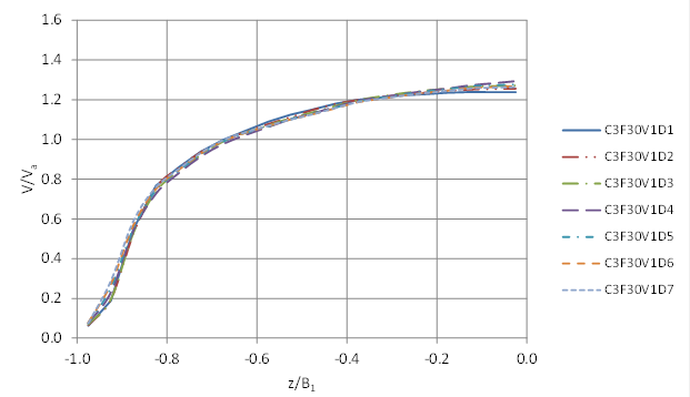
Figure 68. Graph. Vertical slice velocity for 30-percent embedment (V1)
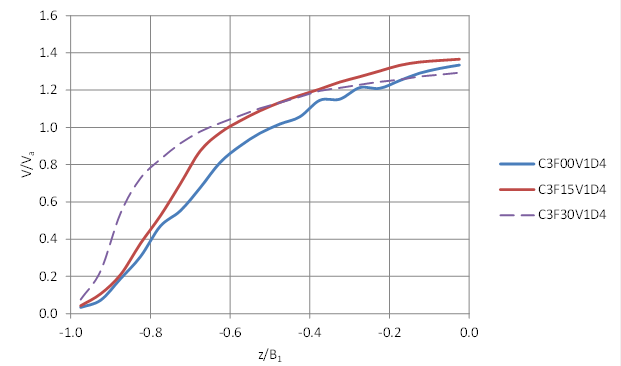
Figure 69. Graph. Vertical slice comparison (V1D4)
A structured approach to parameter estimation is conducted while respecting the physical meaning of the parameters. Parameters are estimated based on the 3-ft culvert CFD runs and validated on the 6- and 8-ft culvert CFD runs. Because the parameters M and βi more fundamentally affect the computation of the isovels, these two parameters are addressed first, starting with M, the velocity distribution parameter related to the maximum point velocity in the cross-section. Once the parameters are fitted to the CFD data, design equations to estimate those parameters are developed.
The maximum point velocity from each CFD run was noted. Zhai provided a relation between the parameter M and the mean and maximum velocities in the channel as shown in figure 70.(32) M may be estimated if the maximum velocity in the channel can be estimated. (Average velocity will be known using standard hydraulics techniques when designing a culvert.)

Figure 70. Equation. Relation of M to velocity
Where:
Va = Average velocity in the channel cross-section, ft/s.
Vmax = Maximum velocity in the channel cross-section, ft/s.
M = Velocity distribution parameter.
Several hypotheses for estimating the ratio of average discharge to maximum discharge were tested, including functions of various dimensionless ratios capturing geometric and hydraulic quantities:
(Top width, T, is equal to B1 + B2. For symmetrical cross-sections, B1 = B2 and T equals 2B1.) (Average flow width, Bavg, equals A/(2ymax).)
The ratio of maximum velocity to average velocity did not exhibit a single relationship to any of the variables noted above for all embedment levels. However, one of the strongest patterns was indicated when plotted against the ratio of T2/A. Figure 71 displays this relation, distinguishing the run series by velocity and embedment. However, the relation is quite different for the C3F00V1 and C3F00V2 series (no embedment) compared with the embedded series with 15-percent (C3F15V1 and C3F15V2) and 30-percent (C3F30V1 and C3F30V2) embedment. A consequence of the embedment is it shifts the flow cross-section wetted perimeter from a circular arc to an almost rectangular shape.
Inspection of figure 71 suggests that each embedment level separately follows an equation of the form: Y = aXb + c. After exploring several alternatives, the ratio B1/Bavg was selected to determine the equation form for estimating the maximum velocity ratio. Figure 72 shows that variation in the maximum velocity ratio is strongly influenced by B1/Bavg and embedment.
These analyses led to the relation for estimating the maximum velocity ratio based only on channel geometry as shown in figure 73. With the equation in figure 73, the parameter M can now be generated using the equation presented in figure 70.
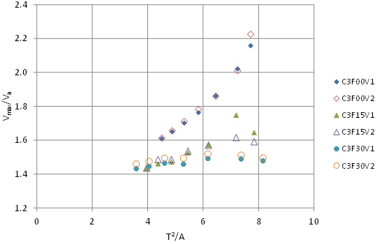
Figure 71. Graph. Variation of Vmax ratio with T2/A
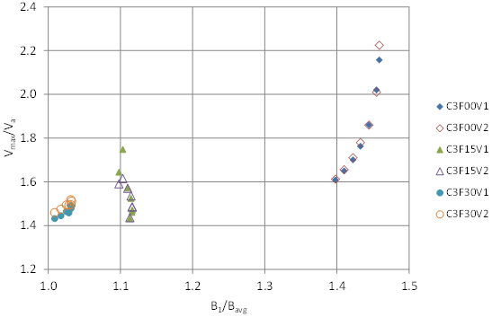
Figure 72. Graph. Variation of Vmax ratio with B1/Bavg

Figure 73. Equation. Estimation of Vmax/Va
Where:
Va = Average velocity in the channel cross-section, ft/s.
Vmax = Maximum point velocity in the channel cross-section, ft/s.
Bavg= Average width for the symmetrical culvert half section, ft.
B1= Maximum top width for the symmetrical culvert half section, ft.
T = Top width for the full section, ft.
A = Cross-section area for the full section, ft2.
Figure 73 assumes that the parameters T and B1 increase as the water surface elevation increases. However, the test matrix includes runs where the two deepest depths with the 30-percent embedment have top widths less than the maximum culvert width (1.1 percent or less). Therefore, relations based on T and B1 may also be applied when the water surface elevation exceeds the elevation of the maximum culvert width as long as T is within two percent of the maximum width.
A comparison of the observed CFD values and those computed using the equation is shown in figure 74. The figure indicates good agreement with one apparent outlier from the C3F15V1 series (C3F15V1D2). The RMSE for the 42 runs included in this analysis was 0.046, which is equivalent to 2.9 percent of the average Vmax/Va ratio.
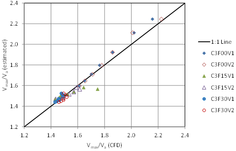
Figure 74. Graph. Calculated versus observed Vmax/Va ratios
Low Velocity Isovel and Maximum Velocity Location Parameters
Estimates of the low velocity isovel parameters (βi,δi, and δy,) and the maximum velocity location parameter (ε) were made for each 3-ft CFD run by minimizing the differences between the velocities produced by the CFD model and estimates using the velocity model in figure 65. Because the CFD runs did not provide velocity output at uniform gridded locations for each run and produced many more individual points than could be effectively analyzed, the CFD data were transformed into a grid system. The flow cross-section for each run was divided into 20 equal sections horizontally and 20 equal sections vertically, creating a grid of identically sized rectangles. CFD data were converted to this 20 by 20 grid to form a uniform gridded representation of the velocity profile. Each run had up to 400 velocity points representing the velocity distribution. The actual number was less than 400 because the flow cross-sections are not rectangular. (Because these grids are stair-stepped and completely enclose the circular culvert, estimated cross-sectional areas are overestimated slightly.) In addition to the grid, 20 vertical flow slices were computed to represent the depth-averaged velocity variation across the section.
Because of its greater effect on the results, the low velocity parameter, βi, was addressed first. While holding δi, δy, and ε equal to zero and using the calculated value of M,βi was estimated for each run by minimizing the RMSE of the grid and slice data. (The most robust estimates resulted when the objective function of the fitting process was to minimize the sum of the RMSE of the grid and slice data.) The parameters δi, δy, and ε were held to zero because odd "optimal" solutions were found for isolated runs when they were allowed to vary simultaneously in the analysis. That is, best-fits that did not correspond to physical reality were observed. For most runs, this process had little effect on the outcome.
Fitted estimates of βi are shown in table 10 (along with the calculated values of M). For the runs with no embedment (C3F00VxDx),βi declines with flow depth and is slightly higher for the higher-velocity runs (V2). The pattern differs for the runs with embedment at 15 percent of the culvert diameter (C3F15VxDx). For these runs, βi increases with flow depth and is slightly higher for the higher-velocity runs. For the runs with embedment at 30 percent (C3F30VxDx),βi is constant at about 1.3. Again, it appears that as the wetted perimeter geometry changes from a circular arc to a rectangular shape, the velocity distribution parameters change accordingly.
Several of the independent variables previously identified were evaluated as possible predictors of βi. Figure 75 displays the relation with the ratio βi/Bavg. There does appear to be another influence on βi in addition to this ratio, especially for the no-embedment and 15-percent embedment runs. Other variables that explained other influence were not identified, perhaps because there is insufficient variation in the range of variables within the 42 CFD runs. This may be further investigated but was not within the scope of this research project. The recommended equation for estimating βi is shown in figure 76.
Figure 77 summarizes the comparison of the fitted values for βi from the CFD and the estimated values using the equation in figure 76. The RMSE for the 42 runs included in this analysis was 0.12, which is equivalent to 6.3 percent of the average value of βi.
Table 10 . Fitted estimates of velocity distribution parameters for the 3-ft culvert.
Run ID |
M |
βi |
δi |
δy |
ε |
|---|---|---|---|---|---|
C3F00V1D1 |
-0.45 |
2.78 |
0.54 |
0.00 |
1.17 |
C3F00V1D2 |
-0.06 |
2.69 |
0.54 |
0.00 |
1.62 |
C3F00V1D3 |
0.45 |
2.63 |
0.59 |
0.00 |
2.59 |
C3F00V1D4 |
0.82 |
2.67 |
0.67 |
0.00 |
3.70 |
C3F00V1D5 |
1.08 |
2.52 |
0.58 |
0.00 |
3.95 |
C3F00V1D6 |
1.31 |
2.48 |
0.68 |
0.00 |
5.37 |
C3F00V1D7 |
1.51 |
2.50 |
0.72 |
0.00 |
6.83 |
C3F00V2D1 |
-0.61 |
2.99 |
0.33 |
0.00 |
0.50 |
C3F00V2D2 |
-0.03 |
2.72 |
0.45 |
0.00 |
1.44 |
C3F00V2D3 |
0.45 |
2.70 |
0.47 |
0.00 |
2.07 |
C3F00V2D4 |
0.75 |
2.73 |
0.57 |
0.00 |
3.02 |
C3F00V2D5 |
1.03 |
2.59 |
0.53 |
0.00 |
3.31 |
C3F00V2D6 |
1.28 |
2.55 |
0.63 |
0.00 |
4.60 |
C3F00V2D7 |
1.49 |
2.57 |
0.68 |
0.00 |
5.89 |
C3F15V1D1 |
1.34 |
1.73 |
0.00 |
0.22 |
0.00 |
C3F15V1D2 |
0.88 |
1.98 |
0.00 |
0.46 |
0.27 |
C3F15V1D3 |
1.71 |
1.97 |
0.00 |
0.32 |
0.00 |
C3F15V1D4 |
1.98 |
2.02 |
0.00 |
0.38 |
0.00 |
C3F15V1D5 |
2.35 |
2.00 |
0.00 |
0.52 |
0.00 |
C3F15V1D6 |
2.42 |
2.12 |
0.00 |
0.51 |
0.00 |
C3F15V1D7 |
2.65 |
2.10 |
0.00 |
0.56 |
0.00 |
C3F15V2D1 |
1.61 |
1.80 |
0.00 |
0.13 |
0.00 |
C3F15V2D2 |
1.48 |
1.89 |
0.00 |
0.19 |
0.05 |
C3F15V2D3 |
1.72 |
1.95 |
0.00 |
0.24 |
0.00 |
C3F15V2D4 |
1.92 |
1.99 |
0.00 |
0.28 |
0.00 |
C3F15V2D5 |
2.25 |
2.09 |
0.00 |
0.45 |
0.00 |
C3F15V2D6 |
2.25 |
2.03 |
0.00 |
0.33 |
0.00 |
C3F15V2D7 |
2.61 |
2.12 |
0.00 |
0.44 |
0.00 |
C3F30V1D1 |
2.30 |
1.29 |
0.00 |
0.01 |
0.00 |
C3F30V1D2 |
2.22 |
1.31 |
0.00 |
0.04 |
0.00 |
C3F30V1D3 |
2.21 |
1.32 |
0.00 |
0.09 |
0.02 |
C3F30V1D4 |
2.44 |
1.40 |
0.00 |
0.07 |
0.05 |
C3F30V1D5 |
2.40 |
1.32 |
0.00 |
0.16 |
0.24 |
C3F30V1D6 |
2.54 |
1.31 |
0.00 |
0.19 |
0.00 |
C3F30V1D7 |
2.64 |
1.31 |
0.00 |
0.21 |
0.00 |
C3F30V2D1 |
2.19 |
1.33 |
0.00 |
0.02 |
0.01 |
C3F30V2D2 |
2.08 |
1.33 |
0.00 |
0.07 |
0.10 |
C3F30V2D3 |
2.03 |
1.34 |
0.00 |
0.14 |
0.19 |
C3F30V2D4 |
2.19 |
1.37 |
0.00 |
0.14 |
0.04 |
C3F30V2D5 |
2.19 |
1.35 |
0.00 |
0.25 |
0.46 |
C3F30V2D6 |
2.32 |
1.34 |
0.00 |
0.25 |
0.08 |
C3F30V2D7 |
2.43 |
1.33 |
0.00 |
0.26 |
0.00 |
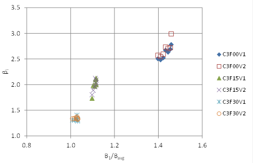
Figure 75. Graph. Variation of βi with B1/Bavg

Figure 76. Equation. Estimation of βi
The remaining three velocity distribution parameters, ε, δi, and δy, were fitted simultaneously, holding the previously determined values of M and βi fixed.δi, and δy were restricted to non-negative values to be consistent with their physical meaning as shown in figure 60 and figure 61. (When allowed to be negative, the optimization rarely selected negative values for these two parameters.)
Initially,ε was allowed to take on any value because it can be negative, zero, or positive. Because ε represents the location of the maximum velocity in the cross-section (positive values are the distance above the water surface, and negative values are the distance below the water surface), the appropriate value of ε may be validated by inspection of the CFD data. In all CFD runs, the maximum velocity was at the surface or increasing when the surface was reached based on the gridded velocities. Therefore,ε was also restricted to non-negative values.
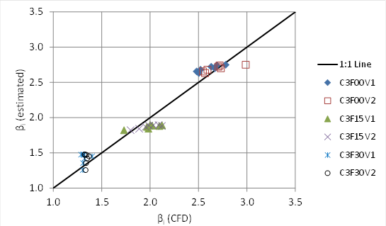
Figure 77. Graph. Estimated versus CFD βi
Figure 78 shows a centerline plot of the middle depth (D4) at each embedment level and velocity level from the 3-ft CFD runs. The profile for no embedment differs significantly from the other embedment levels. This differentiation in profile caused by the cross-section changes results in significant differences in the fitted values of the parameters ε, δi, and δy. The zero embedment cases are the furthest removed from a rectangular-shaped flow cross-section.
Any approach for estimating ε must recognize the differing velocity profiles shown in figure 78. For the no-embedment cases (C3F00), the velocity appears to be increasing slightly as the water surface is approached, suggesting that for these cases, ε should be greater than zero in accordance with the velocity distribution model shown in figure 60. The values reported in table 10 confirm this observation.
Similarly, the velocity profiles for the 15- and 30-percent levels of embedment indicate that maximum velocity is reached at or near the surface, meaning thatε should be zero. For most runs, zero was obtained in the optimization for the C3F15 and C3F30 series. Several runs resulted in small negative values of ε that made only nominal improvements in the fit of the profiles to the CFD results. These values were forced to zero.
The fitted estimates for δi and δy are also summarized in table 10. For the runs with no embedment, the best fit values of δy were all zero, with nonzero values of ε and δi. For these runs, using these nonzero values significantly reduced prediction errors for the gridded and slice velocity estimates. Conversely, for the runs with 15-percent and 30-percent embedment, the best fit values of δy were all nonzero, with zero values of δi in all cases. For these runs, using the nonzero values did not significantly reduce prediction errors for the gridded and slice velocity estimates.
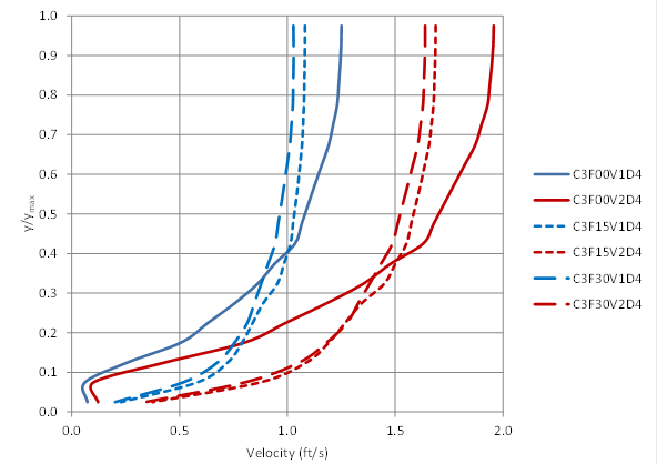
Figure 78. Graph. Velocity profiles for the D4 depth
For the no-embedment runs, several relations were explored as a basis for estimating ε. Two variables identified for further analysis were the T2/A ratio (see figure 79) and the Froude number (see figure 80). Both show decreases in ε, normalized by the maximum flow depth, with increases in the respective variable. However, for a given value of the T2/A ratio, the lower-velocity runs (V1) result in a higher normalized ε , while for a given value of the Froude number, the lower-velocity runs result in a lower normalized ε.
Combining these observations, the behavior of the no-embedment cases may be estimated using the equation in figure 81. For the 15- to 30-percent embedment cases, ε is zero. For more general application, the ratio B1/Bavg is used as the means of distinguishing embedment levels. When B1/Bavg is greater than or equal to 1.2, the equation in figure 81 applies; otherwise,ε is zero.
Figure 82 summarizes the comparison of the fitted values for ε/ymax from the CFD and the estimated values using the equation in figure 81. The RMSE for the 14 runs included in this analysis was 0.057, which is equivalent to 13.4 percent of the average value of ε/ymax.
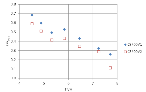
Figure 79. Graph. Variation ofε with T2/A
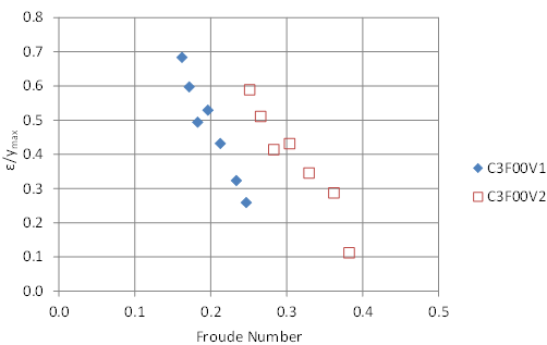
Figure 80. Graph. Variation of ε with Froude number

Figure 81. Equation. Estimation of ε for B1/Bavg ≥ 1.2
Where:
ε = Velocity profile parameter, ft.
ymax = Flow depth at the y axis (culvert centerline), ft.
Fr = Froude number based on average cross-section velocity and depth.
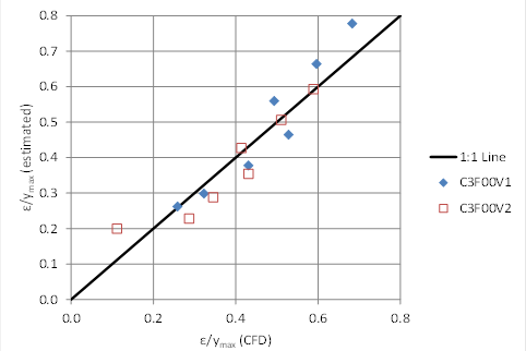
Figure 82. Graph. Estimated versus CFD for ε/ymax
The final two parameters defining the cross-section velocity distribution are the horizontal and vertical offsets. The parameter δi represents a horizontal offset adjustment in the computation of Z as defined in figure 64. This parameter is needed to better fit the isovels on the culvert sides in the no-embedment case. The parameter δi equals zero in every 15- and 30-percent embedment case. Therefore, when B1/Bavg is less than 1.2, δi is set to zero. When B1/Bavg is greater than or equal to 1.2, δi is estimated by the equation in figure 83.
![]()
Figure 83. Equation. Estimation of δi for B1/Bavg ≥ 1.2
The parameter δy represents a vertical offset adjustment to the computation of Y as defined in figure 63, which is needed to better fit the isovels on the culvert bottom in the embedment cases. δi equals zero in every no-embedment case. When B1/Bavg is greater than or equal to 1.2, δi is set to zero. For the 15- and 30-percent embedment cases, adjustment of this parameter does not significantly improve the velocity profile fits. However, the equation in figure 84 may be used.
![]()
Figure 84. Equation. Estimation of δi for B1/Bavg < 1.2
Where:
δi = Velocity profile parameter, ft.
ymax = Flow depth at the y axis (culvert centerline), ft.
ay = Constant dependent on embedment.
The constant, ay, depends on the degree of embedment as measured by the B1/Bavg ratio and is summarized in table 11. For the zero embedment case, ay is zero and δy is zero. For those cases with a nonzero δy,the value of ay goes down with the ratio of B1/Bavg.
Table 11. Summary of embedment constant ay.
B1/Bavg |
Embedment |
ay |
|---|---|---|
<1.06 |
30 percent |
0.018 |
< 1.2 and > 1.06 |
15 percent |
0.050 |
> 1.2 |
0 percent |
0.000 |
It follows from the design equations for estimating δi and δy that ξ0 must equal zero in all design situations addressed in this research report. For the case where B1/Bavg is less than 1.2,δy equals zero, and Y (computed from the equation in figure 63) will be zero at the centerline of such a channel at the bed elevation (z = 0 and i = 0). Similarly, for the case where B1/Bavg is greater than or equal to 1.2, δy equals zero, and Z (computed from the equation in figure 64) will be zero at the channel edge at the water surface elevation (|z|= B1 and y = ymax). Because either Y or Z must equal zero in all cases, there is a value of ξ that will equal zero, according to the equation in figure 62. Therefore, the minimum value of ξ (that is, ξ0) is zero.
The RMSE expressed as a percentage of the average velocity for each run were calculated for the velocity distribution grid. Each velocity in the 20 by 20 grid as modeled by CFD was compared to the velocity at that location using the velocity model with the fitted (best-fit) parameters in table 10. Similarly, each velocity in the 20 by 20 grid as modeled by CFD was compared to the velocity generated by the velocity model with the parameters estimated by the proposed design equations. These errors are summarized in table 12 as "Fitted: Grid" and "Estimated: Grid," respectively.
Errors were also computed on the depth-averaged slices. These errors were computed using both the fitted (best-fit) parameters as well as the parameters estimated using the proposed design equations. Table 12 summarizes these results.
Table 12. Summary of RMSE estimates for the 3-ft culvert runs.
Category |
Minimum (percent) |
Median (percent) |
Maximum (percent) |
|---|---|---|---|
Fitted: Grid |
5.3 |
10.1 |
26.4 |
Estimated: Grid |
5.6 |
10.7 |
25.9 |
Fitted: Slice |
2.2 |
3.4 |
6.9 |
Estimated: Slice |
2.2 |
4.4 |
10.6 |
As expected, the errors using the design equations (estimated) are higher than those using the fitted parameters, but not significantly. It should be noted that for a few runs, either the grid or slice RMSE for the estimated parameters is lower than the RMSE for the fitted parameters. Recalling that the fitting used the sum of the grid and slice RMSE as the objective function, it is possible for one to decrease with the estimated parameters, but the sum of the two decreases. A complete list of RMSE results is in appendix A.
Figure 85 illustrates the slice velocities for the run with the highest fitted slice RMSE (6.9 percent). This run (C3F00V2D1) has no embedment, the higher velocity, and the shallowest depth (0.37 ft). The slice velocities predicted by the fitted and estimated parameters are nearly identical. However, they both overpredict velocity in a portion of the culvert and underpredict the depth-averaged velocity near the centerline. Inspection of the CFD data, however, suggests the mapping of the CFD data to the grid might be improved.
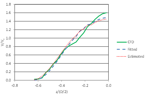
Figure 85. Graph. Comparison of velocities for C3F00V2D1
More typical results are provided in figure 86 and figure 87, which depict runs C3F00V2D6 and C3F30V2D6, respectively. Run C3F00V2D6 has no embedment, the higher velocity, and the sixth-deepest depth (0.75 ft). Generally, the runs for the no-embedment cases have the higher RMSE values, possibly because the geometry of these runs is the full rounded culvert.
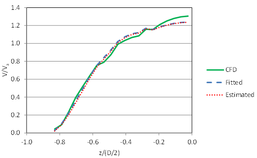
Figure 86. Graph. Comparison of velocities for C3F00V2D6
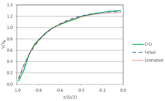
Figure 87. Graph. Comparison of velocities for C3F30V2D6
Run C3F30V2D6 has the greatest embedment (30 percent of the culvert diameter), the higher velocity, and the sixth-deepest depth (0.75 ft). Generally, the runs with the highest embedment cases have the lowest RMSE values, possibly because the geometry of these runs is nearly rectangular. The differences in the no-embedment and 30-percent embedment cases were frequently critical to the development of the design equations.
The design equations were developed based on the analyses of the 3-ft culvert CFD runs. These equations were validated using the 6- and 8-ft CFD runs. The 6-ft runs are scaled based on the Froude number from the 3-ft runs. The scaling was performed to test the utility of the CFD modeling but will have value in validating the design equations. The 8-ft runs are not scaled and represent a more independent set of validation data.
Fitted parameters were determined for the 6-ft culvert runs using the same approach described for the 3-ft culvert runs. These parameters are summarized in table 13. Data were not available for one run and are labeled "n/a" for "not available." Table 14 summarizes the minimum, median, and maximum RMSE for the 6-ft runs for the fitted parameters and the parameters estimated from the design equations. As expected and previously observed with the 3-ft culvert runs, the errors using the design equations (estimated) are higher than those using the fitted parameters, but not significantly. The RMSE errors for the 6-ft culvert runs are comparable to the RMSE errors for the 3-ft culvert runs, as expected. A complete listing of RMSE results for the 6-ft culvert runs is found in appendix A.
Table 13. Fitted estimates of velocity distribution parameters for the 6-ft culvert.
Run ID |
M |
βi |
δi |
δy |
ε |
|---|---|---|---|---|---|
C6F00V1D1 |
-0.53 |
3.02 |
0.19 |
0.00 |
0.40 |
C6F00V1D2 |
0.27 |
2.97 |
0.63 |
0.00 |
1.85 |
C6F00V1D3 |
1.27 |
2.62 |
1.20 |
0.00 |
7.00 |
C6F00V2D1 |
-0.33 |
2.66 |
0.20 |
0.00 |
0.80 |
C6F00V2D2 |
0.24 |
2.90 |
0.88 |
0.00 |
2.89 |
C6F00V2D3 |
1.23 |
2.57 |
1.28 |
0.00 |
8.03 |
C6F15V1D1 |
1.33 |
1.83 |
0.00 |
0.39 |
0.00 |
C6F15V1D2 |
1.62 |
1.96 |
0.00 |
0.68 |
0.00 |
C6F15V1D3 |
2.49 |
2.15 |
0.00 |
1.28 |
0.00 |
C6F15V2D1 |
1.31 |
1.80 |
0.00 |
0.33 |
0.00 |
C6F15V2D2 |
1.65 |
1.94 |
0.00 |
0.62 |
0.00 |
C6F15V2D3 |
2.49 |
2.13 |
0.00 |
1.19 |
0.00 |
C6F30V1D1 |
2.29 |
1.35 |
0.00 |
0.03 |
0.00 |
C6F30V1D2 |
1.80 |
1.29 |
0.00 |
0.31 |
0.42 |
C6F30V1D3 |
2.52 |
1.30 |
0.00 |
0.18 |
0.00 |
C6F30V2D1 |
n/a |
n/a |
n/a |
n/a |
n/a |
C6F30V2D2 |
2.53 |
1.36 |
0.00 |
0.16 |
0.00 |
C6F30V2D3 |
2.39 |
1.30 |
0.00 |
0.22 |
0.08 |
Table 14. Summary of RMSE estimates for the 6-ft culvert runs.
Category |
Minimum (percent) |
Median (percent) |
Maximum (percent) |
|---|---|---|---|
Fitted: Grid |
5.7 |
11.7 |
23.5 |
Estimated: Grid |
5.8 |
11.8 |
22.7 |
Fitted: Slice |
2.5 |
3.9 |
6.7 |
Estimated: Slice |
2.4 |
5.5 |
7.9 |
The runs shown in figure 88 and figure 89 are the scaled versions of the runs presented in the discussion of the 3-ft culvert analyses. Run C6F00V2D3 has no embedment, the higher velocity, and the deepest depth (1.5 ft) of this series. (The drop in the CFD slice velocity in the last slice, which is closest to the culvert centerline, reflects CFD output in the shallow depths that is lower in this slice than in the adjacent slice.)
Run C6F30V2D3 has the greatest embedment (30 percent of the culvert diameter), the higher velocity, and the deepest depth (1.5 ft). Generally, these runs with the highest embedment cases have the lowest RMSE values, possibly because the geometry of these runs is nearly rectangular. These results confirm the observations using the 3-ft culvert runs.
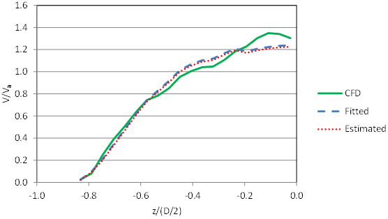
Figure 88. Graph. Comparison of velocities for C6F00V2D3
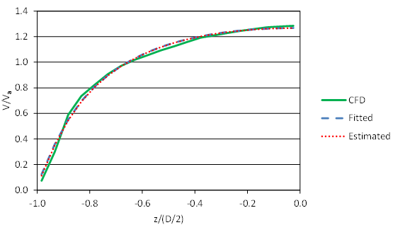
Figure 89. Graph. Comparison of velocities for C6F30V2D3
Fitted parameters were determined for the 8-ft culvert runs using the same approach described for the 3-ft culvert runs. These parameters are summarized in table 15. Data were not available for several runs, which are labeled "n/a" for "not available." Table 16 summarizes the minimum, median, and maximum RMSE for the 8-ft runs for the fitted parameters and the parameters estimated from the design equations. As expected and previously observed with the 3-ft and 6-ft culvert runs, the errors using the design equations (estimated) are higher than those using the fitted parameters, but not significantly. Caution is appropriate in evaluating this table because it includes results from only 6 of the 18 runs in the experimental matrix. The other runs were not completed because of schedule or budget limitations. A complete listing of RMSE results, including a list of the runs completed for the 8-ft culvert runs, is found in appendix A.
The runs shown in figure 90 and figure 91 are not scaled from the 3-ft culvert but have the same relative embedment and flow depths as the runs presented in the discussions of the 3- and 6-ft culvert analyses. Run C8F00V2D3 has no embedment, the higher velocity, and the deepest depth (2.0 ft) of this series. Run C8F30V2D3 has the greatest embedment (30 percent of the culvert diameter), the higher velocity, and the deepest depth (2.0 ft). Generally, these runs with the highest embedment cases have the lowest RMSE values, possibly because the geometry of these runs is nearly rectangular. These results confirm the observations using the 3-ft and 6-ft culvert models.
Table 15 . Fitted estimates of velocity distribution parameters for the 8-ft culvert.
Run ID |
M |
βi |
δi |
δy |
ε |
|---|---|---|---|---|---|
C8F00V1D1 |
n/a |
n/a |
n/a |
n/a |
n/a |
C8F00V1D2 |
n/a |
n/a |
n/a |
n/a |
n/a |
C8F00V1D3 |
n/a |
n/a |
n/a |
n/a |
n/a |
C8F00V2D1 |
n/a |
n/a |
n/a |
n/a |
n/a |
C8F00V2D2 |
n/a |
n/a |
n/a |
n/a |
n/a |
C8F00V2D3 |
1.82 |
2.66 |
1.69 |
0.00 |
15.58 |
C8F15V1D1 |
1.69 |
1.63 |
0.00 |
0.02 |
0.06 |
C8F15V1D2 |
n/a |
n/a |
n/a |
n/a |
n/a |
C8F15V1D3 |
1.77 |
2.11 |
0.00 |
1.02 |
0.29 |
C8F15V2D1 |
n/a |
n/a |
n/a |
n/a |
n/a |
C8F15V2D2 |
n/a |
n/a |
n/a |
n/a |
n/a |
C8F15V2D3 |
2.28 |
2.06 |
0.00 |
0.50 |
0.00 |
C8F30V1D1 |
n/a |
n/a |
n/a |
n/a |
n/a |
C8F30V1D2 |
n/a |
n/a |
n/a |
n/a |
n/a |
C8F30V1D3 |
2.07 |
1.38 |
0.00 |
0.94 |
0.00 |
C8F30V2D1 |
n/a |
n/a |
n/a |
n/a |
n/a |
C8F30V2D2 |
n/a |
n/a |
n/a |
n/a |
n/a |
C8F30V2D3 |
2.27 |
1.27 |
0.00 |
0.15 |
0.03 |
n/a = not available.
Table 16 . Summary of RMSE estimates for the 8-ft culvert runs.
Category |
Minimum (percent) |
Median (percent) |
Maximum (percent) |
|---|---|---|---|
Fitted: Grid |
4.8 |
8.6 |
18.5 |
Estimated: Grid |
5.3 |
10.7 |
17.9 |
Fitted: Slice |
2.0 |
2.8 |
7.4 |
Estimated: Slice |
2.8 |
5.0 |
9.5 |
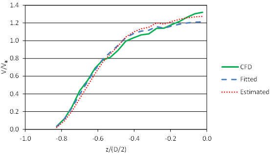
Figure 90. Graph. Comparison of velocities for C8F00V2D3
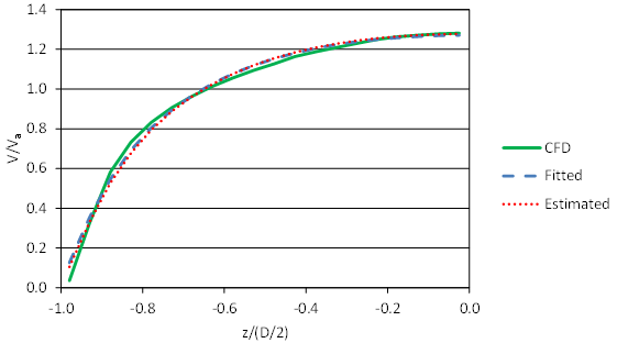
Figure 91. Graph. Comparison of velocities for C8F30V2D3
Application of the design equations is illustrated with two examples. In both cases, the objective is to determine the portion of the culvert that can pass a particular fish requiring flow velocity less than 1.3 ft/s and flow depth of at least 0.5 ft. The design discharge in both examples is the high passage discharge, QH, which equals 7.8 ft3/s. The slope of the stream at the culvert crossing is 0.0015 ft/ft, which is also to be used as the slope of the culvert barrel.
The tailwater channel is approximated by a trapezoidal channel with a bottom width of 5.5 ft and 1:1 side slopes. The bed material has a D50 of 0.944 inches with a D84 of 2.6 inches. Assuming normal depth (0.88 ft) in the tailwater channel and using the Blodgett method, a Manning's roughness of 0.033 is estimated for the bed material.
In this example, a 6-ft diameter corrugated metal pipe (CMP) embedded to a depth of 2 ft is evaluated. (HEC 26 recommends minimum embedment of 30 percent of the culvert diameter or 2 ft, whichever is larger.)(1) The configuration is shown in figure 92. The Manning's roughness for the culvert is 0.028 according to HDS 5.(18) Because the embedment material will be the same material as that found in the tailwater channel, a Manning's n of 0.033 is used for the embedment.
Using a culvert analysis tool such as HY-8, the hydraulic properties within the culvert for the given conditions are determined. Normal depth is 0.91 ft, but HY-8 shows that this depth is not reached within the culvert barrel under these conditions. The depth in the barrel ranges from 0.88 ft at the culvert outlet (controlled by the tailwater depth) to a slightly deeper 0.89 ft at the culvert inlet. For consideration of fish passage, the lower depth (higher velocity) condition at the outlet is used. From the HY-8 output, the average velocity at the outlet is 1.51 ft/s. The average velocity exceeds the velocity specified for the fish of interest, suggesting this configuration is a barrier to passage.
The methods developed in this report are applied to determine whether this is true. Estimates of the following quantities and parameters are required:
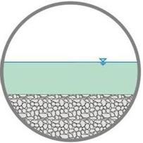
Figure 92. Illustration. Embedded culvert for example 1
To determine the velocity distribution within the culvert, the parameters M, βi, δi, δy, and ε must be estimated. To do this, a few ratios describing the situation are required: T2/A and B1/Bavg. To develop these, one needs to compute A, T, B1, and Bavg as follows:
A = Q/V = 7.8/1.51 = 5.17ft2
For a circular conduit, the water surface top width T is calculated from figure 93.
![]()
Figure 93. Equation. Water surface top width
Where:
Θ = Angle between a line to the water surface at the edge of the pipe from the center of the pipe to the vertical.
![]()
Figure 94. Equation. Angle to water surface
Where:
de = Embedment depth, ft (m).
In this example, ymax = y = 0.88 ft; de = 2.0 ft; and D = 6.0 ft.
Θ = acos(1 - 2(0.88 + 2.0)/6) = 87.7 degrees
T = 6.0 sin(87.7) = 6.0ft.
For the symmetrical pipe, B1 = T/2 = 6.0/2 = 3.0 ft.
Bavg = (A/2)/ymax = (5.17/2)/0.88 = 2.94ft
T2/A = (6.0)2/5.17 = 6.96
B1/Bavg = 3.0/2.94 = 1.02
Estimate Velocity Distribution Parameters
Next, the velocity distribution parameters are estimated:
Vmax/Va is calculated from the equation in figure 73:
Vmax/Va = [0.047 - 0.029(1.02)][6.96][-2.7 + 3.6(1.02)]+1.38 = 1.50
From this, Vmax = 1.5 Va = 1.5 (1.51) = 2.26 ft/s.
M is calculated from the equation in figure 70:
Va/Vmax = 0.667 = eM/(eM-1) - 1/M
By trial and error, M is calculated as 2.19.
βi is calculated from the equation in figure 76:
βi = 2.56(B1 / Bavg - 1)0.49 + 1 = 2.56(1.02 - 1)0.49 + 1 = 1.39
For this example, B1/Bavg is less than 1.2. Therefore, ε and δi are both set to zero.
The final parameter, δy, is calculated using the equation in figure 84 with ay = 0.018 taken from table 11:
δy = ayymax = 0.018(0.88) = 0.016 ft
The final parameters needed are the minimum and maximum isovel values. The minimum value, ξ0, represents the lowest velocity zone, which occurs at the channel perimeter. In the design cases covered by this methodology, ξ0 equals zero.
The maximum value, ξmax, represents the highest velocity zone in the cross-section. Because ε ≥ 0, the maximum occurs at the centerline of a symmetrical cross-section (z = 0) at the water surface when y = ymax, as illustrated in figure 60. The corresponding values of Y, Z, and ξ are estimated from the equations in figure 63, figure 64, and figure 62, respectively:
Y = (y + δy)/(ymax = δy + ε) = (0.88 + 0.016)/(0.88 + 0.016 + 0) = 1.0
Z = |z|/(Bi + δi) = |0|/(3.0 + 0) = 0
ξ = Y(1 - Z)βiexp(βiZ - Y + 1) = 1.0(1 - 0.0)1.39exp(1.39(0) - 1.0 + 1) = 1.0
From the above, ξmax = 1.0.
Example Computation of a Point Velocity
With the above parameters specific to this example, velocities throughout the flow field can be computed. The velocity at a point 0.5 ft above the bed and 1.0 ft to the left of the culvert centerline, shown in figure 95, is computed to demonstrate the process.
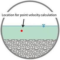
Figure 95. Illustration. Location for example 1 point velocity computation
For this computation, y = 0.5 ft and z = -1.0 ft. The value for the isovel,ξ, is computed the same way as ξmax was computed using the equations in figure 63, figure 64, and figure 62, respectively:
Y = (y + δy)/(ymax + δy + ε) = (0.5 + 0.016)/(0.88 + 0.016 + 0) = 0.576
Z = |z|/(Bi + δi) = |-1|/(3.0 + 0) = 0.333
ξ = Y(1 - Z)βiexp(βiZ - Y + 1) = 0.576(1 - 0.333)1.39exp(1.39(0.333) - 0.576 + 1) = 0.796
With this information, one calculates the point velocity from the equation in figure 65:
V = 1/M ln[1 = (eM - 1) ξ - ξ0 / (ξmax - ξ0] Vmax = 1/2.19 ln[1 + (e2.19 - 1) 0.796 - 0/(1 - 0)] 2.26 = 2.05 ft/s
Therefore, the estimated velocity at a point in the flow field 0.5 ft above the bed and 1.0 ft to the left of the culvert centerline is 2.05 ft/s.
Estimating the Overall Velocity Distribution
To evaluate the entire cross-section, point velocities may be computed on a rectangular grid, such as the 20 by 20 grid used in previous analyses. Slice velocities can then be computed by depth-averaging the grid point values. The result of this process for example 1 is summarized in table 17. The slices are numbered from the left edge of the flow cross-section looking downstream through the culvert. Higher velocities are observed moving to the right toward the culvert centerline. Because this cross-section approximates a rectangular shape, the depth after slice 1 is constant at 0.88 ft. Velocity and depth are shown graphically in figure 96.
For the design criteria (velocity ≤ 1.3 ft/s and depth ≥ 0.5 ft), this design satisfies the depth requirement across the entire width of the flow cross-section except a narrow part of slice 1. However, the velocity criterion is met for only the six leftmost slices because the velocity in these slices is less than 1.3 ft/s. Passage is facilitated when both criteria are satisfied. For this case, both criteria are satisfied in the six leftmost slices. Because each slice represents a width of 0.15 ft (B1 divided by 20), 0.9 ft of flow width (6 times 0.15) meets the design criteria for passage, allowing for passage to occur even though the average velocity suggests that would not be the case. Because the culvert and flow field are symmetrical, a mirror image passage path also exists on the right side.
Table 17 . Slice velocity and depths for example 1.
Slice Number |
Distance from Centerline (ft) |
Velocity (ft/s) |
Depth (ft) |
|---|---|---|---|
1 |
-2.92 |
0.16 |
0.57 |
2 |
-2.77 |
0.46 |
0.88 |
3 |
-2.62 |
0.74 |
0.88 |
4 |
-2.47 |
0.96 |
0.88 |
5 |
-2.32 |
1.14 |
0.88 |
6 |
-2.17 |
1.28 |
0.88 |
7 |
-2.02 |
1.40 |
0.88 |
8 |
-1.87 |
1.50 |
0.88 |
9 |
-1.72 |
1.58 |
0.88 |
10 |
-1.57 |
1.65 |
0.88 |
11 |
-1.42 |
1.70 |
0.88 |
12 |
-1.27 |
1.75 |
0.88 |
13 |
-1.12 |
1.79 |
0.88 |
14 |
-0.97 |
1.82 |
0.88 |
15 |
-0.82 |
1.84 |
0.88 |
16 |
-0.67 |
1.86 |
0.88 |
17 |
-0.52 |
1.88 |
0.88 |
18 |
-0.37 |
1.89 |
0.88 |
19 |
-0.22 |
1.90 |
0.88 |
20 |
-0.07 |
1.90 |
0.88 |
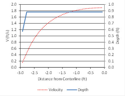
Figure 96. Graph. Velocity and depth for example 1
Example 2: Non-embedded Culvert
In this example, a 6-ft diameter CMP without embedment is evaluated. The configuration is shown in figure 97. There is no bed material within the culvert, and the Manning's roughness for the culvert is 0.028 according to HDS 5.(18)
Using a culvert analysis tool, such as HY-8, the hydraulic properties within the culvert for the given conditions are determined. Normal depth is 1.27 ft, but HY-8 shows that this depth is not reached within the culvert barrel under these conditions. The depth in the barrel ranges from 0.88 ft at the culvert outlet (controlled by the tailwater depth) to 1.14 ft (approaching normal) at the culvert inlet. For consideration of fish passage, the lower depth (higher velocity) condition at the outlet is used. From the HY-8 output, the average velocity is 3.01 ft/s at the culvert outlet. The average velocity exceeds the velocity specified for the fish of interest, suggesting this configuration is a barrier to passage.
The methods developed in this report are applied to determine whether this is true. Estimates of the following quantities and parameters are required:
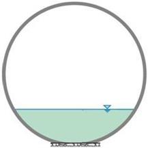
Figure 97. Illustration. Culvert without embedment for example 2
To determine the velocity distribution within the culvert, the parameters M, βi, δi, δy, and ε must be estimated. To do this, a few ratios describing the situation are required: T2/Aand B1/Bavg. To develop these one needs to compute A, T, B1, and Bavg as follows:
A = Q/V = 7.8/3.01 = 2.59 ft2
For a circular conduit, the water surface top width T is calculated from the equations in figure 93 and figure 94. In this example, ymax = y = 0.88 ft; de = 0.0 ft; and D = 6.0 ft.
Θ = acos (1 - 2(0.88 + 0.0)/6) = 45.0 degrees
T = 6.0 sin(45.0) = 4.24 ft
For the symmetrical pipe, B1 = T/2 = 4.24/2 = 2.12 ft
Bavg = (A/2)/ymax = (2.59/2)0.88 = 1.47 ft
T2/A = (4.24)2/2.59 = 6.94
B1/Bavg = 2.12/1.47 = 1.44
Estimate Velocity Distribution Parameters
Next, the velocity distribution parameters are estimated:
Vmax/Va is calculated from the equation in figure 73:
Vmax/Va = [0.047 - 0.029(1.44)][6.94][-2.7 = 3.6(1.44)] + 1.38 = 2.02
From this, Vmax = 2.02 Va = 2.02 (3.01) = 6.08 ft/s.
M is calculated from the equation in figure 70:
Va/Vmax = 0.495 = eM/(eM - 1) - 1/M
By trial and error, M is calculated as -0.12.
Î’i is calculated from the equation in figure 76:
βi = 2.56(B1/(Bavg) - 1)0.49 + 1 = 2.56(1.44 - 1)0.49 + 1 = 2.71
For this example, B1/Bavg is greater than or equal to 1.2. Therefore, ε is nonzero. To estimate ε, the Froude number based on average cross-section velocity and depth (ya = A/T) is required:
Fr = Va/(√(gya)) = 3.01/(√(32.2(2.59/4.24))) = 0.68
Using the equation in figure 81,ε is calculated as follows:
ε = 2.56(T2/(A))-1.54 (Fr)-0.62 ymax = 2.56(6.94)-1.54 (0.68)-0.62 0.88 = 0.14
Because B1/Bavg is greater than or equal to 1.2, the equation in figure 83 is used to calculate δi as follows:
δi = 0.04B1 = 0.04(2.12) = 0.085
Because B1/Bavg is greater than or equal to 1.2, the final parameter, δy, is set equal to zero.
The final parameters needed are the minimum and maximum isovel values. The minimum value, ξ0, represents the lowest velocity zone, which occurs at the channel perimeter. In the design cases covered by this methodology, ξ0 equals zero.
The maximum value, ξmax, represents the highest velocity zone in the cross-section. Because ε ≥ 0, the maximum occurs at the centerline of a symmetrical cross-section (z = 0) at the water surface when y = ymax as illustrated in figure 60. The corresponding values of Y, Z, and ξ are estimated from the equations in figure 63, figure 64, and figure 62, respectively.
Y = (y + δy)/(ymax + δy + ε) = (0.88 + 0.0)/(0.88 + 0.0 + 0.14) = 0.863
Z = |z|/(Bi + δi) = |0|/(2.12 + 0.085) = 0
ξ = Y(1 - Z)βiexp(βiZ - Y + 1) = 0.863(1 - 0.0)2.71exp(2.71(0) - 0.863 + 1) = 0.99
From the above, ξmax = 0.99.
Example Computation of a Point Velocity
With the above parameters specific to this example, velocities throughout the flow field can be computed. The velocity at a point 0.5 ft above the bed and 1.0 ft to the left of the culvert centerline, shown in figure 98, is computed to demonstrate the process.
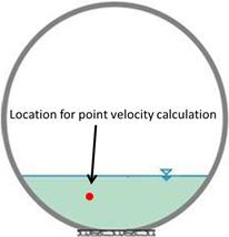
Figure 98. Illustration. Location for example 2 point velocity computation
For this computation, y = 0.5 ft and z = -1.0 ft. The value for the isovel, ξ, is computed the same way as ξmax was computed using the equations in figure 63, figure 64, and figure 62, respectively:
Y = y + δy / ymax + δy + ε = 0.5 + 0.0 / 0.88 + 0.0 + 0.14 = 0.490
Z = |z|/(Bi + δi) = |-1|/(2.12 + 0.085) = 0.453
ξ = Y(1 - Z)βiexp(βiZ - Y + 1) = 0.490(1 - .453)2.71exp(2.71(0.453) - 0.490 + 1) = 0.543
With this information, one calculates the point velocity from the equation in figure 65:
V = 1/M ln[1 = (eM - 1) ξ - ξ0 / (ξmax - ξ0] Vmax = 1/-0.12 ln[1 + (e-0.12 - 1) 0.543 - 0/(0.99 - 0)] 6.08 = 3.2 ft/s
Therefore, the estimated velocity at a point in the flow field 0.5 ft above the bed and 1.0 ft to the left of the culvert centerline is 3.2 ft/s.
Estimating the Overall Velocity Distribution
To evaluate the entire cross-section, point velocities may be computed on a rectangular grid, such as the 20 by 20 grid used in previous analyses. Slice velocities can then be computed by depth-averaging the grid point values. The result of this process for example 2 is summarized in table 18. The slices are numbered from the left edge of the flow cross-section looking downstream through the culvert. Higher velocities are observed moving to the right toward the culvert centerline. Depth is shown graphically in figure 99, and velocity is shown in figure 100.
For the design criteria (velocity ≤ 1.3 ft/s and depth ≥ 0.5 ft), this design does not meet the depth requirement in the first six slices of the flow cross-section. However, the depth is sufficient for passage to the right of this point as shown in figure 99. The velocity criterion is met only for the five leftmost slices, as seen in figure 100. For passage to occur, both criteria must be satisfied in the same area of the culvert. Therefore, in this case there is no part of the flow field that satisfies both the depth and velocity criteria; the flow velocity is too high, the flow depth is too low, or both (as in slice 6). Therefore, this culvert is a fish passage barrier.
Table 18. Slice velocity and depths for example 2.
Slice Number |
Distance from Centerline (ft) |
Velocity (ft/s) |
Depth (ft) |
|---|---|---|---|
1 |
-2.07 |
0.04 |
0.04 |
2 |
-1.96 |
0.16 |
0.13 |
3 |
-1.86 |
0.37 |
0.22 |
4 |
-1.75 |
0.66 |
0.31 |
5 |
-1.65 |
1.00 |
0.40 |
6 |
-1.54 |
1.39 |
0.44 |
7 |
-1.43 |
1.76 |
0.53 |
8 |
-1.33 |
2.16 |
0.57 |
9 |
-1.22 |
2.53 |
0.62 |
10 |
-1.11 |
2.87 |
0.66 |
11 |
-1.01 |
3.16 |
0.70 |
12 |
-0.90 |
3.39 |
0.75 |
13 |
-0.80 |
3.55 |
0.79 |
14 |
-0.69 |
3.81 |
0.79 |
15 |
-0.58 |
3.86 |
0.84 |
16 |
-0.48 |
4.03 |
0.84 |
17 |
-0.37 |
4.16 |
0.84 |
18 |
-0.27 |
4.07 |
0.88 |
19 |
-0.16 |
4.13 |
0.88 |
20 |
-0.05 |
4.15 |
0.88 |
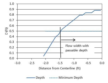
Figure 99. Graph. Depth for example 2
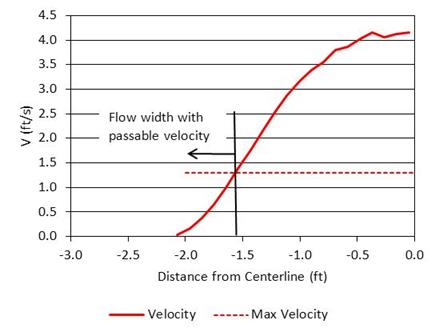
Figure 100. Graph. Velocity for example 2
Both design examples show cross-section average velocities in excess of the maximum required velocity for the target fish. Using the same culvert size in both cases, the case without embedment (example 2) provides no locations where both depth and velocity criteria are met. However, using the same culvert with 2.0 ft of embedment, a passable width in the culvert is provided. It is important to note that this culvert is sunk 2.0 ft in example 1 compared with example 2.
The designer should repeat these analyses at the low passage flow, QL. The high and low passage flows bracket when passage is likely to be required. These flows may be specified by the appropriate regulatory agency to specifically correspond with the fish species of interest. The designer should also verify that the embedded culvert retains sufficient capacity to satisfy the applicable peak flow requirements.
It should be noted that the combination of the depth and embedment in example 1 forces the water surface above the culvert spring line, where further increases in depth will result in a decrease in top width, T. The design equations were not developed for relative depths above those included in this study and should be used with caution for depths above the spring line. However, because the decrease in width is within the 2-percent guideline provided previously, the use of these equations is valid in this example.
In addition, this methodology focuses on the main culvert barrel, not the inlet and outlet where flow transitions will modify the velocity profile. Other complicating factors could include the presence of debris and nonuniform bed conditions within the culvert.
VELOCITY DESIGN CHART DEVELOPMENT (CHANG'S METHOD)
The design equations and applications previously demonstrated can be applied using computer aided tools, for example, spreadsheets or custom software. When such tools are unavailable, the simplified design charts provided in this section may be used. There will be some loss of accuracy, but application is accomplished without advanced tools.
The design charts are derived from the concepts that Dr. Fred Chang developed when this research project was being developed. Chang hypothesized that a generalized series of curves describing the ratio of the cumulative cross-section average velocity from the left edge of the culvert to the cross-section average velocity could be developed. A conceptual example is shown in figure 101.
Chang suggested that such a tool could be used to estimate the fish path width, given the average culvert velocity and the fish passage velocity. For example, if the average culvert velocity is 1.5 ft/s and the maximum fish passage velocity is 1.3 ft/s, then such a tool can be used to find the portion of the culvert cross-section that averages 1.3 ft/s. To do so, the designer would take the ratio of 1.3/1.5 = 0.87 and enter the design chart on the ordinate axis at this value. One would read an abscissa value of approximately -0.3. This means that the average cross-sectional velocity from the left edge of the water surface in the culvert to this point is 1.3 ft/s. The fish passage width, therefore, is the leftmost 70 percent of the flow width. If the culvert is symmetrical at its center, then there would be a mirror image fish passage path on the right side of the culvert.
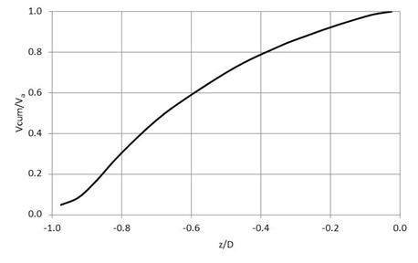
Figure 101. Graph. Conceptual cumulative velocity relation
However, this approach overestimates the fish passage width because the average velocity includes vertical slices that are less than the average (toward the left edge) and vertical slices that are greater than the average (toward the culvert center). Therefore, this entire width is not available for fish passage.
This problem is addressed by considering the vertically averaged velocities directly rather than cumulative averages as described in the previous section of this report. (This approach will still produce some vertical slices where the velocities near the surface exceed the fish passage velocity, but this occurrence is reduced compared with the cumulative approach discussed in this section.)
Given this limitation, the data available from this study were analyzed, and it was determined that four design curves could reasonably represent the range of circular culvert conditions studied. These four design curves are summarized as follows:
These curves are shown graphically in figure 102 and in table 19. These curves were selected after examining the CFD runs for differences based on Froude numbers, Reynolds numbers, and the geometrical ratios T/D and B1/Bavg. Although the CFD data included culvert diameters between 3 and 8 ft, inclusively, the dimensionless curves should be applicable to larger culverts.
No data were developed in this study for box shapes. However, design curve 4 may be used for boxes because the flow cross-section shapes for higher levels of embedment closely approximate a rectangular shape. This curve applies for all levels of embedment in box shapes.
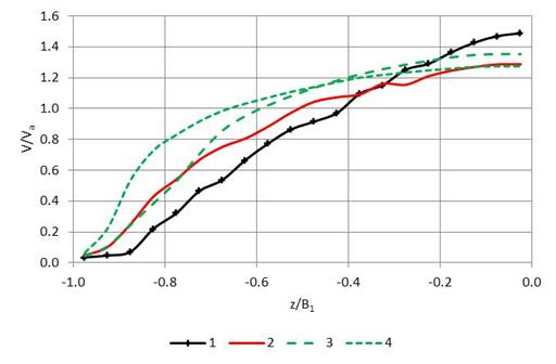
Figure 102. Graph. Vertical slice design curves
Using the values from the previous illustration (average culvert velocity = 1.5 ft/s and the maximum fish passage velocity = 1.3 ft/s), one can find the portion of the culvert cross-section that has vertical slices with velocities less than or equal to 1.3 ft/s. With this approach, one would also have to know more about the site condition. It is assumed that this is a culvert with 30-percent embedment; therefore, design curve 4 is the appropriate choice. By inspection of either table, the ratio of 0.87 (1.3/1.5) is exceeded in vertical slice 6. That means that the first five slices provide velocities less than fish passage velocity. Because each slice represents one-twentieth of one half of the water surface flow width, the fish passage width is the leftmost 25 percent (5 times 1/20) of the flow width from the left edge to the culvert centerline. The same result is obtained by using the figure. Use of these design curves is also illustrated in the application guide provided in appendix C of this document.
Table 19 . Tabular listing of vertical slice design curves.
Slice |
z/B1 |
V/Va |
V/Va |
V/Va |
V/Va |
|---|---|---|---|---|---|
1 |
-0.975 |
0.036 |
0.048 |
0.043 |
0.064 |
2 |
-0.925 |
0.047 |
0.103 |
0.108 |
0.225 |
3 |
-0.875 |
0.072 |
0.252 |
0.246 |
0.537 |
4 |
-0.825 |
0.221 |
0.430 |
0.386 |
0.729 |
5 |
-0.775 |
0.322 |
0.542 |
0.529 |
0.830 |
6 |
-0.725 |
0.465 |
0.667 |
0.705 |
0.917 |
7 |
-0.675 |
0.537 |
0.751 |
0.857 |
0.985 |
8 |
-0.625 |
0.666 |
0.806 |
0.951 |
1.032 |
9 |
-0.575 |
0.774 |
0.884 |
1.021 |
1.071 |
10 |
-0.525 |
0.865 |
0.974 |
1.081 |
1.108 |
11 |
-0.475 |
0.915 |
1.044 |
1.134 |
1.140 |
12 |
-0.425 |
0.972 |
1.073 |
1.182 |
1.172 |
13 |
-0.375 |
1.097 |
1.092 |
1.222 |
1.201 |
14 |
-0.325 |
1.153 |
1.160 |
1.256 |
1.218 |
15 |
-0.275 |
1.253 |
1.155 |
1.285 |
1.235 |
16 |
-0.225 |
1.291 |
1.211 |
1.310 |
1.248 |
17 |
-0.175 |
1.366 |
1.246 |
1.332 |
1.259 |
18 |
-0.125 |
1.428 |
1.269 |
1.348 |
1.270 |
19 |
-0.075 |
1.470 |
1.287 |
1.353 |
1.274 |
20 |
-0.025 |
1.488 |
1.287 |
1.353 |
1.274 |
The analyses and tools from this study are based on round corrugated metal culverts with and without embedment. However, extension of these tools to other situations is possible.
Pipe Arch, Elliptical, and Box Shapes
As described in HDS 5, metal culverts are also available in pipe arch, elliptical, and box shapes, which also have the potential to serve as embedded culverts.(18) As was observed in the analyses of the embedded circular culverts, the flow area approximates a rectangle in many of the cases tested. Therefore, it is reasonable to assume that these methods are applicable to box shapes. These methods may also apply to elliptical culverts.
However, pipe arch shapes have the characteristic that at very low combinations of embedment and flow depth, the top width of the flow field decreases with increasing water surface elevation. Such an occurrence is outside the range of most tests and not well suited for the velocity distribution model that assumes increasing top width with increasing depth. For those conditions in a pipe arch where this is true, the tools developed in this study are considered applicable. For conditions beyond this, the method is not recommended.
The design methods developed for this study rely primarily on the average velocity and cross-section geometry of the flow field. Nothing in the study, particularly the variation in bed material roughness, indicates that the methods are restricted to metal culverts. In addition, analyses were provided for computing a composite roughness for an embedded culvert that are equally applicable to concrete embedded culverts. Therefore, the methods developed for this study are anticipated to be applicable to concrete culverts.
Ledges for Terrestrial Organisms
A series of CFD runs were conducted to evaluate potential effects on the velocity distribution and composite roughness of various ledge configurations intended to provide a dry passage through the culvert for terrestrial organisms. Two alternative configurations were considered-a shelf ledge and a bench ledge-as illustrated in figure 103 and figure 104, respectively. In both cases, the design objective is to provide passage for terrestrial organisms simultaneously with fish passage. Therefore, the top of the ledge should be at or above the water surface elevation for the high passage flow.
For the shelf ledge, the shelf will have little or no influence on the velocity distribution in the flow field, depending on the means of support for the shelf. At flood flows, where the ledge is submerged, the designer should consider the loss of conveyance and increased drag resulting from the presence of the shelf.
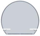
Figure 103. Illustration. Shelf ledge configuration
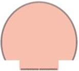
Figure 104. Illustration. Bench ledge configuration
For the bench ledge, the bench eliminates conveyance for both passage and flood flows. As can be seen in figure 104, the remaining cross-sectional area for flow rates with a water surface elevation less than or equal to the top elevation of the bench (fish passage flows) is a rectangular area. Therefore, the methods in this report can be used to evaluate the velocity distribution. As with the shelf ledge, during flood flows when the ledge is submerged, the designer should consider the loss of conveyance and increased drag resulting from the presence of the bench.
Manning's n computations were made for the ledge configurations within an 8-ft CSP pipe with 15-percent embedment. The bed material was represented by a single layer of spheres with a diameter of 2.28 inches. The flow conditions were for full flow with a velocity of 1 ft/s.
For the shelf ledge configuration shown in figure 103, the composite roughness was estimated at 0.028. For the same conditions without the ledge, the composite roughness was estimated at 0.030. An increase is counterintuitive because the presence of the ledge should increase roughness. One possible explanation is that the ledge is represented in the CFD model with no roughness.
For the bench ledge configuration shown in figure 104, the composite roughness was estimated at 0.029. In this case, the bench surfaces are also modeled without roughness, so it is expected that the results would be similar to the shelf ledge. It should be noted that this configuration has a lower cross-sectional area. Because the CFD runs were performed with constant velocity, the bench ledge configuration run represents a lower discharge than was analyzed for the shelf ledge.
Results for both ledge configurations are on the low side of expectations for an 8-ft CSP with a gravel bed material and a ledge. Previous CFD runs for the 8-ft CSP flowing full without embedment resulted in a Manning's n of 0.0325. Therefore, the roughness values for the ledge runs are considered inconclusive.